Analysis of Load Frequency Control Problem for Interconnected Power System Using PID Controller

(1)

International Journal of Emerging Technology and Advanced Engineering

Website: www.ijetae.com (ISSN 2250-2459,ISO 9001:2008 Certified Journal, Volume 4, Issue 11, November 2014)

276

Analysis of Load Frequency Control Problem for

Interconnected Power System Using PID Controller

Dharmendra Jain

1

, Dr. M. K. Bhaskar

2

, Shyam K. Joshi

3

, Deepak Bohra

4

1,4

PG Scholar, 2Associate Professor, Dept. of EE, M.B.M. Engineering College, JNVU, Jodhpur, Rajasthan, India

3_{PhD Scholar, Dept. of EE, IIT Dehli, Dehli, India}

Abstract— This paper present the analysis of load frequency control problem for interconnected power system using the PID controller. Any small sudden load change in any of the areas causes the fluctuation of the frequencies of each and every area and also there is fluctuation of power in tie line of interconnected power system. Frequency should remain nearly constant for satisfactory operation of a power system because frequency deviations can directly impact on a power system operation, system stability, reliability and efficiency. Large frequency deviations can damage equipments, degrade load performance, overload transmission lines and affect the performance of system protection schemes. A Load Frequency Control (LFC) scheme basically incorporates an appropriate control system for an interconnected power system, which is heaving the capability to bring the frequencies of each area and the tie line powers back to original set point values or very nearer to set point values effectively after the sudden load change. This can be achieved by the use of conventional and modern controllers. In this proposed research work PID controller has been applied for LFC of two area power systems. The parameters of the PID controller are tuned by three different methods names as Ziegler-Nichols (Z-N) Method, Simplex Search Method and IMC method for better results. It is seen that the results obtained are far better than the conventional controller.

Keywords— IMC, LFC, PID, set point, Tie line.

I. INTRODUCTION

If there is interconnection exists between two or more control areas through tie line than that is called multi-area interconnected power system. Large size is one of the most important advantages for the whole interconnected power system. When a load block is added, at the initial time, the required energy is temporarily borrowed from the system kinetic energy. Generally the availability of energy is more for larger systems. So there is comparatively less static frequency drop, whereas for a single area power system, the frequency drop may be a bit higher for same amount in load change.

As the peak demands do not have any certain time, they may occur at any random time of the day in many areas, for a large power system the ratio between load peak and load average is smaller as compared to smaller systems. Therefore it is obvious that all interconnected power system areas may benefit from a decreased need of capacity reserved by the scheduled arrangement of interchanging energy.

The generators in a control area always vary their speed together (speed up or slow down) for maintaining the frequency and the relative power angles to the predefined values with tolerance limit in both static and dynamic conditions. If there is any sudden change in load occurs in any control area of an interconnected power system then there will be frequency deviation as well as tie line power deviation. Frequency should remain nearly constant for satisfactory operation of power system. Frequency deviations can directly impact on a power system operation, system reliability and efficiency. Large frequency deviations can damage equipments, degrade load performance, overload transmission lines and affect the performance of system protection schemes. These large-frequency deviation events can ultimately lead to a system collapse. Variation in frequency adversely affects the operation and speed control of induction and synchronous motors.

In domestic appliances, where refrigerator‘s efficiency goes down, television and air conditioners reactive power consumption increases considerably with reduction in power supply frequency. So it is very important to maintain the frequency within acceptable range. Due to the dynamic nature of the load, continuous load change cannot be avoided but the system frequency can be kept within sufficiently small tolerance levels by adjusting the

generation continuously. According to Dr. M. S. Krishnarayalu et.al [20], practically all power

(2)

International Journal of Emerging Technology and Advanced Engineering

277

Basic problems of MAPS are Automatic Generation Control (AGC) which controls the system frequency and Automatic Voltage Regulator (AVR) that keeps system voltage constant at rated value.

Nizamuddin et.al [1] present dynamic modeling for Automatic Generation Control of two area interconnected power system considering diverse sources in each area. The two areas are interconnected by AC tie- line.

II. LOAD FREQUENCY CONTROL

Imbalances between load and generation must be corrected within seconds to avoid frequency deviations that might threaten the stability and security of the power system. The problem of controlling the frequency in large power systems by adjusting the production of generating units in response to changes in the load is called load frequency control (LFC). The Objectives of LFC are to provide zero steady-state errors of frequency and tie-line exchange variations, high damping of frequency oscillations and decreasing overshoot of the disturbance so that the system is not too far from the stability. The load frequency control of a multi area power system generally incorporates proper control system, by which the area frequencies could brought back to its predefined value or very nearer to its predefined value so as the tie line power, when the is sudden change in load occurs.

The above mentioned objectives are carried out successfully in previous works by different researchers using Fuzzy logic, PI and PID controllers, optimal control, Variable structure control, adaptive and self-tuning control etc.

Modern control techniques provide great help in LFC of power systems. Now days there are more complex power systems and required operation in less structured and uncertain environment. Similarly innovative and improved control is required for economic, secure and stable operation. Modern control techniques are having the ability to provide high adaption for changing conditions. They are having the ability for making quick decisions. Many researchers are working in this area.

The standard definitions of the different terms for LFC of power system are heaving the approval by the IEEE STANDARDS Committee in 1968[17]. The dynamic model suggestions were described thoroughly by IEEE PES working groups [17, 18]. On the basis of experiences with real implementation of LFC schemes, various modifications to the ACE definition were suggested time to time to cope with the changing environment of power system.

III. PIDCONTROLLER

The PID control scheme is named after its three correcting terms, whose sum constitutes the manipulated variable (MV). The proportional, integral, and derivative terms are summed to calculate the output of the PID controller. Defining U(t) as the controller output, the final form of the PID controller is given in equation (1).

U(t) = MV(t) = KP e(t) + Ki ∫ dt + Kd

…(1)

A.Proportional Term

The proportional term produces an output value that is proportional to the current error value. The proportional response can be adjusted by multiplying the error by a constant Kp, called the proportional gain constant. The proportional term is given in equation (2).

Output = Pout = KP e(t) .... (2)

B.Integral Term

The contribution from the integral term is proportional to both the magnitude of the error and the duration of the error. The integral in a PID controller is the sum of the instantaneous error over time and gives the accumulated offset that should have been corrected previously. The accumulated error is then multiplied by the integral gain Ki and added to the controller output. The integral term is given by equation (3).

Iout = Ki ∫ dt ….. (3) The integral term accelerates the movement of the process towards set point and eliminates the residual steady-state error that occurs with a pure proportional controller. However, since the integral term responds to accumulated errors from the past, it can cause the present value to overshoot the set point value.

C.Derivative Term

The derivative of the process error is calculated by determining the slope of the error over the time and multiplying this rate of change by the derivative gain Kd. The magnitude of the contribution of the derivative term to the overall control action is termed the derivative gain, Kd. The derivative term is given by equation (4).

(3)

International Journal of Emerging Technology and Advanced Engineering

278

Derivative action predicts system behaviour and thus improves settling time and stability of the system. An ideal derivative is not causal, so that implementations of PID controllers include an additional low pass filtering for the derivative term to limit the high frequency gain and noise. Derivative action is seldom used in practice because of its variable impact on system stability in real-world applications.

In the early history of automatic process control the PID controller was implemented as a mechanical device. These mechanical controllers used a lever, spring and a mass were often energized by compressed air. These pneumatic controllers were the industry standard at that time.

After development of mechanical controller researchers were working on the new controllers. As a result of their research they have developed the electronic analog controller. Electronic analog controllers can be made from a solid-state or tube amplifier or from a capacitor and a resistor. Electronic analog PID control loops were often found within more complex electronic systems, for example, the head positioning of a disk drive, the power conditioning of a power supply or even the movement-detection circuit of a modern seismometer. Nowadays, electronic controllers have largely been replaced by digital controllers implemented with microcontrollers or FPGAs.

Most modern PID controllers in industry are implemented in programmable logic controllers (PLCs) or as a panel-mounted digital controller. Software implementations have the advantages that they are relatively cheap and are flexible with respect to the implementation of the hardwares. PID temperature controllers are applied in industrial ovens, plastic injection machinery, hot stamping machines and packing industry.

It is necessary to adjust the parameters of PID controller to obtain the desired response.

IV. TUNING OF PIDCONTROLLER

Tuning: Tuning a control loop is the adjustment of its control parameters (proportional gain, integral gain and derivative gain) to the optimum values for the desired control response. Stability (no unbounded oscillation) is a basic requirement, but beyond that, different systems have different behaviour, different applications have different requirements and requirements may conflict with each other.

PID tuning is a difficult problem even though there are only three parameters and its principle is simple to describe, because it must satisfy complex criteria within the limitations of PID control.

There are accordingly various methods for tuning and more sophisticated techniques are the subject of patents. This section describes some methods for tuning of controller parameters in PID controllers, that is, methods for finding proper values of Kp, Ki and Kd.

Designing and tuning a PID controller appears to be conceptually intuitive, but can be hard in practice, if multiple and often conflicting objectives such as short transient and high stability are to be achieved. PID controllers often provide acceptable control using default tunings, but performance can generally be improved by careful tuning and performance may be unacceptable with poor tuning. Usually, initial designs need to be adjusted repeatedly through computer simulations until the closed-loop system performs as desired.

A. Ziegler-Nichols (Z-N) Closed-Loop Tuning Method

The Ziegler-Nichols closed-loop tuning method allow to use the ultimate gain value Ku and the ultimate period of oscillation Tu, to calculate Kp . It is a simple method of tuning PID controllers and can be refined to give better approximations of the controller. The controller constants Kp, Ki and Kd can be obtained for a system with feedback. Determining the ultimate gain value Ku is accomplished by finding the value of the proportional gain that causes the control loop to oscillate indefinitely at steady state. This means that the gains from the I and D controller are set to zero so that the influence of P can be determined. It tests the robustness of the Kp value so that it is optimized for the controller. Another important value associated with this proportional control tuning method is the ultimate period (Tu). The ultimate period is the time required to complete one full oscillation while the system is at steady state. These two parameters, Ku and Tu, are used to find the loop-tuning constants of the controller (P, PI, or PID). To find the values of these parameters and to calculate the tuning constants, use the following procedure:

1. Remove integral and derivative action. Set integral gain (Ki) to zero value and set the derivative controller gain (Kd) to zero.

2. Create a small disturbance in the loop by changing the set point. Adjust the proportional, increasing and/or decreasing, the gain until the oscillations have constant amplitude.

3. Record the gain value (Ku) and period of oscillation (Tu).

(4)

International Journal of Emerging Technology and Advanced Engineering

279

TABLE1

PIDCONTROLLER PARAMETERS USING Z-NMETHOD

Control Type Kp Ki Kd

P 0.5 Ku - -

PI 0.45 Ku 1.2Kp/Tu -

PD 0.8 Ku - Kp Tu /8

PID 0.60 Ku 2Kp/ Tu Kp Tu /8

PID controller parameters calculated using Ziegler– Nichols Method are given in Table 2.

TABLE2

PIDCONTROLLER PARAMETERS CALCULATED USING Z-NMETHOD

Power system area-1 Power system area-2

Ku Tu Kp Ki Kd Ku Tu Kp Ki Kd

1.1 4s 0.66 0.33 0.33 1.5 4s 0.9 0.45 0.45

B. Tuning of PID Controller By Simplex Search Method

Tuning of PID controller parameters can be done with the help of simulation software. Simulation software are very popular now a days. Simplex search method is one of the methods of tuning the PID controller parameters using simulation in MATLAB. When a Simulink model is design in MATLAB simulink to meet requirements for optimizing parameters, MATLAB simulink design optimization software automatically converts the requirements into a constrained optimization problem and then solves the problem using optimization techniques. The constrained optimization problem iteratively simulates the simulink model, compares the results of the simulations with the constraint objectives and uses optimization methods to adjust tuned parameters to better meet the objectives.

The results obtained from Simplex tuning method are shown in Table 3.

TABLE3

PIDCONTROLLER PARAMETERS OBTAINED USING SIMPLEX METHOD

Kp Ki Kd Kp Ki Kd

0.4221 1.2113 0.3295 0.9 0.45 0.45

C. Internal Model Control Tuning of PID Controller

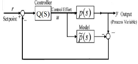
Internal model control (IMC) is one of the recent methods of tuning. IMC is a popular control structure in process control. The IMC structure given by Garcia & Morari, 1982 is shown in Figure 1.

[image:4.612.59.280.156.234.2]

It is the main part of the design of controllers. Its conceptual usefulness lies in the fact that it allows to concentrate on the controller design without having to be concerned with control system stability provided that process model ̃(s) is a perfect representation of stable process P(s).

Fig. 1: Internal Model Control (IMC) configuration

The IMC design procedure goes as follows:

Decompose the plant model ̃(s) into two parts one is invertible (minimum phase) part PM(s) and other is all pass

(Non minimum phase) part PA(s) with unity magnitude as

shown in equation (5).

̃(s) = PM(s) PA(s) ….(5)

Design a set point-tracking IMC controller as given in equation (6).

... (6)

Where is a tuning parameter such that the desired set point response is 1/( s+1)r, and r is the relative degree of PM(s).

It is shown that IMC control can achieve very good tracking performance. However, the load disturbance rejection performance sometimes is not satisfactory. So a second controller is added to improve the disturbance-rejection performance. A disturbance-rejecting IMC controller Qd is given in equation (7).

Qd(s) = (1 s+1)/( d s+1) …. (7)

Where d is a tuning parameter for disturbance rejection,

m is the number of poles of P(s) such that the Qd(s) needs

to cancel and 1 can be given as in equation (8).

 ( ) ( ) …. (8)

[image:4.612.331.564.215.324.2] [image:4.612.42.296.287.358.2] [image:4.612.41.296.583.650.2]

(5)

International Journal of Emerging Technology and Advanced Engineering

[image:5.612.59.273.137.229.2]

280

Fig. 2 : Equivalent conventional feedback configuration

Where, K is feedback controller. The feedback controller K can be given as shown in equation (9).

….. (9)

The standard procedure for obtaining tuned PID controller parameters from IMC controllers is to expand the final controller into Maclaurin series and get the coefficients of the first three terms. The procedure can be obtained from the IMCTUNE package [12]. Wen Ten [12, 13] is working in the area of LFC with PID controller using different methods for tuning of parameters. Wen Ten is discussed as a future work in one of his research paper is that PID controller parameters can be tuned and approximate PID controller can be obtained from frequency domain.

The method is proposed in this work for tuning of PID controller parameters as follows.

The procedural steps are described as:

Step-1: Given any controller K(s), get a frequency range of interest, compute the frequency response of K(s).

Step-2: Find the frequency wm such that the magnitude

of K(jw) achieves its minimum value.

Step-3: Then the approximated PID is given in equation (10).

KPID(s) = KP + Ki/s + Kd s ….. (10)

Where, KP = Real part of K(jwm) ... (11)

Ki = K(jws)lwb ….. (12)

Kd = Real part of K(jwm) - Ki/ jwm ….. (13)

Where wb is very small frequency (like wb=0.01 or any

other suitable value). The procedure amounts to approximating K(s) by a PID controller with the same integral action and the lowest turning point and the resulted PID controller retains the magnitude of the IMC controller at low to medium frequency range, thus the load-rejecting performance will be guaranteed to that of the IMC controller.

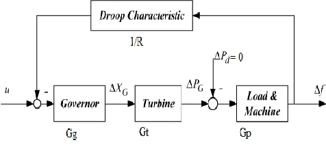
LFC Design with Droop Characteristic

Droop characteristics is a feedback gain to improve the damping properties of the power system, and it is generally set to 1/R before load frequency control design, so in this case the block diagram for LFC can be given as fig.3.

Fig.3 : Linear model of a single-area power system with droop characteristics.

System can be given as equation (14). P(s) =

…. (14)

Where, Governor with dynamics: Gg(s) = 1/(1+ sTG)

Turbine with dynamics: Gt(s) = 1/(1+ sTT) and

Load and machines with dynamics: GP(s) = KP/(1+ sTP)

V. NUMERICAL ANALYSIS

Two power systems with non-reheat turbine with the droop characteristics have been taken. The model parameters are given in table 4.

Using the parameters given in table 4 and the equation (14), power system for area-1 and area-2 are obtained as shown in equation (15) and equation (16) respectively.

P1(s) = 1.67/(1.67s3+11.8s2+17.4s+34.4) …. (15)

P2(s) = 1.67/(1.6s3+8.16s2+9.78s+18.76) …. (16)

Final controller can be obtained using the equation (9) with the values of Q(s), Qd(s) and P(s) from equation (6),

equation (7) and equation (14) respectively.

Bode plots for K1(s) and K2(s) are shown in fig.4 and

[image:5.612.325.563.206.315.2]

(6)

International Journal of Emerging Technology and Advanced Engineering

281

TABLE4

PARAMETERS OF POWER SYSTEM AREA-1 AND AREA-2

S. No Parameter

power

system

area-1

power

system

area-2

1 Speed Regulation due to governor action R (Hz/p.u.MW)

0.05 0.0625

2 Frequency sensitive load coefficient D

0.6 0.9

3 Inertia Constant H 5 4

4 Base Power (MVA) 1000 1000

5 Governor Time Constant TG (Ʈg) 0.2 s 0.3 s

6 Turbine Time Constant TT (Ʈt) 0.5 s 0.6 s

7 Electric System Gain KP =(1/D) 1.67 1.11

8 Electric System Time Constant TP 16.7 8.88

Fig. 4 : Bode plot for K(s) for power system area-1

Fig. 5 : Bode plot for K(s) for power system area-2

The PID controller parameters obtained from IMC tuning method are shown in Table 5.

TABLE5

PIDCONTROLLER PARAMETERS OBTAINED USING IMCMETHOD

Kp Ki Kd Kp Ki Kd

2.4457 1.5847 1.5267 2.4110 1.4255 1.5055

VI. RESULTS AND DISCUSSION

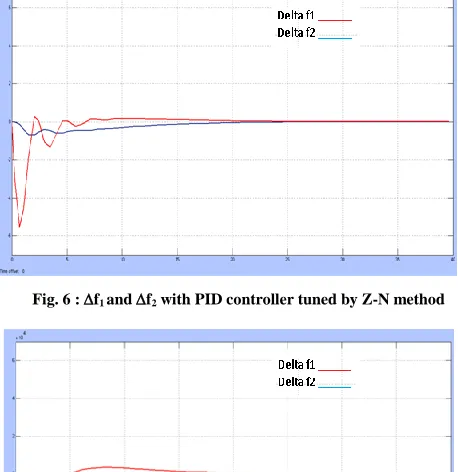
[image:6.612.45.293.133.670.2]

In this section simulated two area interconnected power system connected by the tie line LFC with PID controller are shown. The PID controller whose parameters are tuned with different methods is applied and results are shown. The change in load powers which are the input disturbances are taken as, PL1 = 0.00 pu, PL2 = 0.01 pu.

Fig. 6 : f1 and f2 with PID controller tuned by Z-N method

[image:6.612.317.571.171.258.2] [image:6.612.330.559.358.594.2]

(7)

International Journal of Emerging Technology and Advanced Engineering

[image:7.612.55.284.137.293.2] [image:7.612.332.567.137.286.2]

282

Fig. 8 : f1 and f2 with PID controller tuned by IMC method

[image:7.612.55.285.255.663.2]

Fig. 9 : Ptie with PID controller tuned by Z-N method

Fig. 10 : Ptie with PID controller tuned by Simplex method

Fig. 11 : Ptie with PID controller tuned by IMC method

TABLE6

TIME RESPONSE SPECIFICATIONS FOR F1

S.No Tuning

Method

Mp TP

Tp

Tr Ts Response

1 Z-N -6.1*10-4 1s 2s 28s Stable

2 Simplex -5.8*10-4 _1s _2s _14s _Stable

3 IMC -3.2*10-4 1s 2s 13s Stable

TABLE7

TIME RESPONSE SPECIFICATIONS FOR F2 S.No Tuning

Method

Mp Tp Tr Ts Response

1 Z-N -1*10-4 2s 28s 28s Stable

2 Simplex -0.9*10-4 2s 3s 14s Stable

3 IMC -0.1*10-4 _1s _18s _18s _Stable

TABLE8

TIME RESPONSE SPECIFICATIONS FOR PTIE

S.No Tuning _Method Mp Tp Tr Ts Response

1 Z-N 1.4*10-3 4s 38s 38s Stable 2 Simplex 1.2*10-3 2s 27s 27s Stable 3 IMC 0.5*10-3 2.5s 23s 23s Stable

[image:7.612.316.570.328.608.2] [image:7.612.54.284.329.526.2]

(8)

International Journal of Emerging Technology and Advanced Engineering

283

Similarly fig. 6, fig.7 and fig. 8 are showing the dynamic responses of deviation in frequency for both the areas (f1 ,f2 ) and fig. 9, fig. 10 and fig. 11 are showing the power deviation in tie line (P-tie) for a power system heaving two control areas with PID controller whose parameters are tuned by Z-N method, Simplex method and IMC method respectively. The change in load powers which are the input disturbances are taken as, PL1 = 0.00 pu, PL2 = 0.01

pu.

VII. CONCLUSION

It is important to keep the power system frequency and the inter area tie line power as close as possible to the scheduled values in interconnected power system. Model of a two area interconnected power system has been developed with different area characteristics for modern and conventional control strategies. It has been shown that the use of PID controller can improve the dynamic performance.

A PID controller calculates an error value as the difference between a measured process variable and a desired set point. The controller attempts to minimize the error by adjusting the process through use of a manipulated variable. The PID controllers are widely used in power system and control systems to damp system oscillations, increase stability and reduce steady state error as they are simple to realize and easily tuned. It is seen that if the proper tuning of parameter of PID controller is done, the area frequencies could brought back to its predefined value or very nearer to its predefined value with acceptable tolerance so as the tie line power in minimum time, when the is sudden change in load occurs .

It can be seen that the IMC tuned PID controller is capable of giving the better results as compared to other two methods.

REFERENCES

[1] Nizzamudin et. al. ‗AGC Of Two Area Interconnected Power System With Diverse Sources In Each Area‘, Journal of Electrical Engineering, pp. 1-8.

[2] O. I. Elgerd and C. Fosha, ‗Optimum megawatt frequency control of multiarea electric energy systems,‘ IEEE Trans. Power App. Syst., vol. PAS-89, no. 4, pp. 556–563, Apr. 1970.

[3] P. Kundur, Power System Stability and Control. New York: McGraw-Hill, 1994.

[4] P.P. Khargonekar, I.R. Petersen, K. Zhou, Robust stabilization of uncertain linear systems: quadratic stabilizability and H control theory, IEEE Trans. AC 35 (1990) 356.

[5] R. K. Cavin, M. C. Budge Jr., P. Rosmunsen, ‗An Optimal Linear System Approach to Load Frequency Control‘, IEEE Trans. On Power Apparatus and System, PAS-90, Nov./Dec. 1971, pp. 2472-2482.

[6] R. K. Green, ‗Transformed automatic generation control,‘ IEEE Trans.Power Syst., vol. 11, no. 4, pp. 1799–1804, Nov. 1996. [7] Ray,G., Prasad ,A.N., Prasad, G.D., A new approach to the design of

robust load- frequency controller for large scale power systems, Electric power System Research 51(1999) 13-22.

[8] Shah,N.N., Kotwal,C.D., The state space modeling of single, two and three area ALFC of Power System using Integral Control and Optimal LQR Control method, IOSR Journal of Engineering, Mar 2012, Vol 2(3), pp:501-510.

[9] T. Kennedy, S.M. Hoyt, and C. F . Abell, ‗Variable, non-linear tie line frequency bias for interconnected systems control ‘, IEEE Ttrans. On Power Systems, Vol. 3, No. 3, August 1988, pp. 1244-1253.

[10] V. Ganesh et. al. ‗LQR Based Load Frequency Controller for Two Area Power System‘ International Journal of Advanced Research in Electrical, Electronics and Instrumentation Engineering Vol. 1, Issue 4, October 2012, pp. 262-269.

[11] V. R. Moorthi and R. P. Aggarawal, ‗Suboptimal and near optimal control of a load frequency control system,‘ Proc. Inst. Elect. Eng., vol. 119, pp. 1653– 1660, Nov. 1972.

[12] W. Tan, ―Tuning of PID load frequency controller for power systems‖, Energy Convers, Manage. vol. 50, no. 6, pp. 1465–1472, 2009.

[13] Wen Ten, ‗Unified Tuning of PID Load Frequency Controller for Power Systems via IMC‘ IEEE Transactions On Power Systems, Vol. 25, No. 1, February 2010, pp. 341-350.

[14] Y. H. Moon, H. S. Ryu, J. G. Lee, and S. Kim, ―Power system load frequency control using noise-tolerable PID feedback,‖ in Proc. IEEE Int. Symp. Industrial Electronics (ISIE), Jun. 2001, vol. 3, pp. 1714–1718.

[15] Yao Zhang ‗Load Frequency Control Of Multiple-Area Power Systems‘, Master Of Science In Electrical Engineering, Cleveland State University, August 2009.

[16] Yogendra Arya, Narendra Kumar, S.K. Gupta, ―Load Frequency Control of a Four- Area Power System using Linear Quadratic Regulator‖, IJES Vol.2 2012 PP.69-76.

[17] A. Khodabakhshian and N. Golbon, ―Unified PID design for load frequency control,‖ in Proc. 2004 IEEE Int. Conf. Control Applications (CCA), Taipei, Taiwan, Sep. 2004.

[18] A. M. Stankovic, G. Tadmor, and T. A. Sakharuk, ‗On robust control analysis and design for load frequency regulation,‘ IEEE Trans. Power Syst., vol. 13, no. 2, pp. 449–455, May 1998.

[19] A. Rubaai and V. Udo, ‗An a daptive control scheme for LFC of multi area power systems. Part I: Identification and functional design, Part-II: Implementation and test results by simulation,‘ Elect. Power Syst. Res., vol. 24, no. 3, pp. 183–197, Sep. 1992.