Hyperspectral Data Dimensionality Reduction Using Hybrid Approach

(1)

International Journal of Emerging Technology and Advanced Engineering

Website: www.ijetae.com (ISSN 2250-2459,ISO 9001:2008 Certified Journal, Volume 4, Issue 5, May 2014)

701

Hyperspectral Data Dimensionality Reduction Using Hybrid

Approach

Amit Panwar

1

, Dr. Annapurna Singh

2

, Dr. H.S Bhaduria

3

1

Research Scholar, 2,3Assistant Professor, Computer Science and Engineering Department, GBPEC, Pauri Garhwal, INDIA Abstract— Hyperspectral data contain a large volume of

information. This abundance of data is hard to exploit due to high computational cost involved in processing this data. Dimensionality reduction deals with transforming high dimensional data in to lower dimensional space without losing significance of the High dimensional data. In this paper, a new methodology has been proposed that is based on existing algorithms. This model uses the advantages of PCA, ICA, and MNF to reduce dimensionality with high classification accuracy. Traditional AVIRIS Indian Pine benchmark dataset has been used for experiment. ENVI is used for dimension reduction. ERDAS Imagine has been used for Classification using Maximum likelihood method.

Keywords— Hyperspectral, Dimensionality reduction, AVIRIS, ENVI, ERDAS imagine

I. INTRODUCTION

With the advancement in remote sensing technology, Sensors nowadays are capable of capturing information in more than 200 narrow contiguous bands. A sensor record simultaneously in several different regions of spectrum, creating multi-images taken at the same time [1]. The region of these spectrum captured are known as ‘BANDS’. Satellite image can be classified in two three categories according to number of bands. Panchromatic images consist of only a few bands [2]. Multispectral images consist of 5 to 15 bands while a hyperspectral image is made up of more than 200 bands [3]. Hyperspectral image is gigantic as compared to few megabytes of multispectral image. Due to this large number of bands a new set of algorithm is required that can exploit this highly rich information.

It has been found that Bands from adjacent wavelength regions of hyperspectral data have high degree of correlation among each other. Thus, the information content can be redundant. Data redundancy is direct consequence of the fact that a high dimensional space is mostly empty [4].

There is a stringent requirement of adequate number of pure training samples to extract information from high dimensional data.

Generally the required number of training samples is linearly related to the dimensionality in case of linear classifier and to the square in case of quadratic classifier [5]. Due to non availability of training tuples the classification accuracy decreases with the increase in dimensionality, also known as Hughes phenomenon or ‘the curse of dimensionality’ [6]. Thus it can be summarized that dimensionality reduction not only lowers the computational cost for exploiting the hyperspectral data but also take care of Hughes phenomenon.

This paper is structured as follows. In Section 2, various dimensionality algorithms is explained in detail. In Section 3 the proposed approach is explained with algorithm. Section 4 consists of dataset used in experiment. Section 5 describes the result of the experiment. Section 6 concludes this paper.

II. RELATED WORK

A number of dimensionality reduction techniques has been proposed by researcher, which may be categorized as either feature extraction or feature selection [7]. Feature extraction techniques map’s high dimensional data into lower dimension using some mathematical transformation function. Each method has unique transformation properties. It creates a new feature set by combining existing feature set. In feature selection a set of feature is chosen with help of a criteria function. These algorithms generally involve a search algorithm and a criterion function. Due to this selection a portion of the original information is always lost [8].

Various feature extraction algorithms for dimensionality reduction has been proposed. Including independent component analysis (ICA) [9], Principal component analysis (PCA) [10], Minimum noise fraction (MNF) [11], Discriminative boundary feature extraction algorithm (DBFE) [7]. These methods require a transformation function that maps high dimensional data in to lower dimensions.

(2)

International Journal of Emerging Technology and Advanced Engineering

702 In the second phase, ICA and PCA are applied on the resultant bands obtained from phase first, and then the corresponding PCA and ICA values of the pixel are combined in one feature vector space. The feature vector is classified with corresponding class label.

A. Principal component analysis (PCA)

PCA transforms the highly correlated high dimensional data into uncorrelated low dimension where the resulting components are orthogonal to each other. These components are arranged according to variance [10]. First component or band has highest data variance and the second PC band contains the second largest variance and so on.

PCA finds a new set of orthogonal axes that have their origin at the data mean and that are rotated to maximize the data variance. Covariance matrix is used as transformation matrix and is defined as:

1

(

i

)(

i

)

N _T

i

x

m x

m

 



r



r



r

(1)

Where

x

r

i is the ith spectral signature,

m

r

denotes the

mean spectral signature and N is the number of pixel in the input image. To find the new orthogonal axes of PCA, Eigen decomposition of the covariance matrix



is performed as:

k k k

a





a



r

(2)

Where



k is the Kth eigen value,

a

r

krepresents the

corresponding eigenvector where K varies from 1 to number of bands. The eigenvector forms the axes of PCA space. The eigenvalues are the measure of variance of the corresponding eigenvector. Larger the amount of variance higher is the information content of the band. Based on variance bands are arranged in decreasing order, the first PC bands are retained because of their large variance. PCA transformation matrix, A is created by choosing the eigenvector corresponding to the maximum eigenvalues and is defined as:

1 2 3

[

|

| ... ]

n

A



a a

r

a

r

a

r

(3)

Where

a a

r

1

|

r

2

|

a

r

3

| ...

a

r

n are the eigenvectors associated with n maximum largest eigen values obtained from the decomposition of the covariance matrix.

B. Minimum Noise Fraction (MNF)

PCA algorithm does not consider noise. It considers only variance of each principal component. However the hyperspectral data is not isotropic it means the noise radiation reaches a location from all direction with equal intensity. MNF transform consist of two consecutive data reduction operations. The first operation consists of estimation of noise in the data represented with correlation matrix. Second operation creates a set of components that contains the variance across all bands in the raw data set [11]. This operation is a standard principal component analysis of the noise whitened data.

C. Independent Component Analysis (ICA)

ICA is a blind source separation technique. It assumes that each band is a linear mixture of independent hidden component and extracts the independent feature using a linear unmixing operation [9]. Suppose we have N statistically independent signals, si(t), i=1,…….,N. let X(t) denotes the original source signal. ICA estimates X(t) by,

s(t)= Ux(t)

(4)

Where u is an unknown matrix called the unmixing matrix. This is a blind source separation algorithm since we do not have any prior information about unmixing matrix, or even on the source themselves.

III. THE PROPOSED MODEL

The proposed approach uses the advantages of MNF, PCA and ICA while neutralizing their disadvantages. The proposed model consists of two phases. In first phase MNF is applied to input hyperspectral data while in second phase PCA and ICA is applied on the output of the first phase. Finally a vector comprising of 20 values, 10 each from ICA and PCA is formed. The resulting vector is then classified by Maximum likelihood classifier.

A.

Algorithm

i. INPUT the original hyperspectral data Y of P pixel and N bands.

ii. Apply MNF using ENVI, the resultant bands are ordered according to signal to noise ratio (SNR).

iii. The first 10 bands are selected as input to another step. iv. Apply PCA to the output of step 3.

v. Apply ICA to the output of step 3.

(3)

International Journal of Emerging Technology and Advanced Engineering

703

Fig1. Average spectral response curve of the class used in experiment

IV. DATASET

The dataset is a mining area of an AVIRIS image

available online at

http://aviris.jpl.nasa.gov/html/aviris.freedata.html. The image consist of 224 bands having 533 pixel and 477 lines. This is 16 bit data collected over mining area in southern Nevada with minerals and little vegetation. The water absorption and noisy bands are removed resulting in 197 final bands for processing. Among the Number of class of mineral available, only 14 are chosen here for further analysis.

V. RESULT AND DISCUSSION

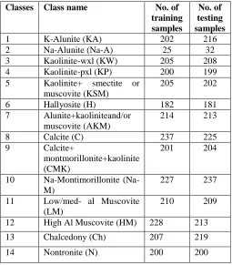
[image:3.612.317.572.417.708.2]

Among available mineral classes available in the dataset, 14 has been used chosen for processing. All the classes, belongs to level IV of Anderson’s classification scheme [12]. Table 1 shows the number of testing and training pixel used for classification. Figure 1 shows the plot of average spectral response curve (SRC) of the classes used for classification versus the number of band available for analysis. Number of training and testing pixel plays vital role in classification. Higher the number of training and testing pixel assures high classification accuracy. Table 2 lists the accuracy of proposed method as well as other method used in experiment.

TABLE I

TRAINING AND TESTING SAMPLES OF THE DATASET

Classes Class name No. of

training samples

No. of testing samples

1 K-Alunite (KA) 202 216 2 Na-Alunite (Na-A) 25 32 3 Kaolinite-wxl (KW) 205 208 4 Kaolinite-pxl (KP) 200 199 5 Kaolinite+ smectite or

muscovite (KSM)

205 202

6 Hallyosite (H) 182 181 7 Alunite+kaoliniteand/or

muscovite (AKM)

214 213

8 Calcite (C) 237 225 9 Calcite+

montmorillonite+kaolinite (CMK)

201 204

10 Na-Montimorillonite (Na-M)

227 237

11 Low/med- al Muscovite (LM)

210 209

12 High Al Muscovite (HM) 228 213

13 Chalcedony (Ch) 207 219

(4)

International Journal of Emerging Technology and Advanced Engineering

[image:4.612.44.570.143.570.2]

704

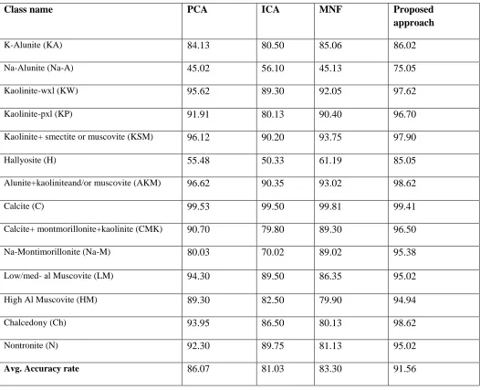
TABLE II

CLASSIFICATION ACCURACY OF PCA, ICA, MNF AND PROPOSED APPROACH

Class name

PCA

ICA

MNF

Proposed

approach

K-Alunite (KA)

84.13

80.50

85.06

86.02

Na-Alunite (Na-A)

45.02

56.10

45.13

75.05

Kaolinite-wxl (KW)

95.62

89.30

92.05

97.62

Kaolinite-pxl (KP)

91.91

80.13

90.40

96.70

Kaolinite+ smectite or muscovite (KSM)

_96.12

_90.20

_93.75

_97.90

Hallyosite (H)

55.48

50.33

61.19

85.05

Alunite+kaoliniteand/or muscovite (AKM)

96.62

90.35

93.02

98.62

Calcite (C)

_99.53

_99.50

_99.81

_99.41

Calcite+ montmorillonite+kaolinite (CMK)

90.70

79.80

89.30

96.50

Na-Montimorillonite (Na-M)

_80.03

_70.02

_89.02

_95.38

Low/med- al Muscovite (LM)

94.30

89.50

86.35

95.02

High Al Muscovite (HM)

89.30

82.50

79.90

94.94

Chalcedony (Ch)

93.95

86.50

80.13

98.62

Nontronite (N)

92.30

89.75

81.13

95.02

Avg. Accuracy rate

86.07

81.03

83.30

91.56

VI. CONCLUSION

From the table 2 we can see that classification accuracy in case of class 2 is higher with ICA, While PCA and MNF work well with large number of training and testing tuples. PCA and MNF are not successful with small class size or with less training and testing tuples. The proposed approach use the advantage of MNF and lists the band according to signal to noise ratio. Further PCA and ICA is applied independently to form the combined feature vector space. Hence as we can see in table 2 the classification accuracy increases with respect to other existing algorithm.

Also the original hyperspectral image is reduced to 20 bands that is good enough take care of Hughes phenomenon.

REFERENCES

[1] Govender, M., K. Chetty, and H. Bulcock. "A review of hyperspectral remote sensing and its application in vegetation and water resource studies." Water Sa33.2 (2007).

[2] Chang, Chein-I., ed. Hyperspectral imaging: techniques for spectral detection and classification. Vol. 1. Springer, 2003.

(5)

International Journal of Emerging Technology and Advanced Engineering

705

[4] Jimenez, Luis O., and David Landgrebe. "High dimensional feature reduction via projection pursuit." ECE Technical Reports (1996): 103.

[5] Fukunaga K. Effect of sample size in classifier design. IEEE Pattern Anal Mach Intell 1989;11(8):873–85.

[6] Hughes, G. "On the mean accuracy of statistical pattern recognizers."Information Theory, IEEE Transactions on 14.1 (1968): 55-63.

[7] Landgrebe DA. Signal theory methods in multispectral remote sensing. Hoboken, New Jersey: John Wiley & Sons; 2003.

[8] BruceLM, YounanNH, KingRL, Cheriyadat. A Spectral reduction image processing techniques. In proceedings of IEEE international

geo science and remote sensing

symposium(IGARSS03),Toulouse,France;21–25th July,2003, vol. 1.p.452–4.

[9] Wang, Jing, and Chein-I. Chang. "Independent component analysis-based dimensionality reduction with applications in hyperspectral image analysis."Geoscience and Remote Sensing, IEEE Transactions on 44, no. 6 (2006): 1586-1600.

[10] Harsanyi, Joseph C., and Chein-I. Chang. "Hyperspectral image classification and dimensionality reduction: an orthogonal subspace projection approach."Geoscience and Remote Sensing, IEEE Transactions on 32.4 (1994): 779-785.

[11] Green, Andrew A., et al. "A transformation for ordering multispectral data in terms of image quality with implications for noise removal." Geoscience and Remote Sensing, IEEE Transactions on 26.1 (1988): 65-74.

[12] Anderson JR. A land use and land cover classification system for use

with remote sensor data,