Thesis by
Xiaojie Gao
In Partial Fulfillment of the Requirements for the Degree of
Doctor of Philosophy
California Institute of Technology Pasadena, California
2008
c
Acknowledgements
First and foremost, it is my great pleasure to thank my advisor Professor Leonard J. Schulman. This thesis would never have existed without his help, support, inspiration, and guidance. To him, I offer my most sincere gratitude.
I wish to thank my fellow members of the theory group for their valuable discus-sions and helpful suggestions for my work.
In addition, my thanks go to Professor K. Mani Chandy, Professor Richard M. Murray, and Professor Chris Umans for helpful discussions. They provided me an education, formally or informally, that will be an invaluable resource in my future career.
I am particularly indebted to my whole family for their love, encouragement, and support, especially my parents who have always been there to offer guidance for me. I owe a lot to my dear husband Chih-Kai Ko, who have helped me in writing on this work and providing constructive suggestions.
Abstract
The Vehicle Routing Problem (VRP) is a discrete optimization problem with high industrial relevance and high computational complexity. The problem has been exten-sively studied since it was introduced by Dantzig and Ramser. In a VRP, we are given a number of customers with known delivery requirements and locations (assumed to be vertices in a network). A fleet of vehicles with limited capacity is available. The objective is to design routes and customer assignments to minimize the total time or distance traveled to serve the demands. Because of its practical significance, this problem has been widely studied.
Contents
Acknowledgements iii
Abstract iv
1 Introduction 1
1.1 Review . . . 2
1.2 Motivation . . . 3
1.3 Problem Statement . . . 4
1.4 Main Contributions . . . 5
2 Off-line Case 7 2.1 Examples . . . 7
2.1.1 Example 1: All Demands Are in a Square . . . 8
2.1.2 Example 2: All Demands Are on a Line . . . 8
2.1.3 Example 3: All Demands Are in a Single Point . . . 8
2.2 Characterization of Optimal Off-line Performance . . . 9
2.3 Approximation Algorithm to Compute Woff. . . 19
3 On-line case 22 3.1 Diffusing Computations . . . 22
3.2 On-line Strategy . . . 23
3.2.1 Vehicle State . . . 25
3.2.2 The Overall Structure . . . 26
3.2.3.1 Messages Used in Phase I . . . 27
3.2.3.2 Local Data Used By a Vehicle During Phase I . . . . 27
3.2.3.3 Phase I Algorithm Description . . . 28
3.2.4 Phase II Computation . . . 29
3.2.5 Discussion . . . 29
3.3 Proof of Theorem 1.4.2 . . . 31
4 Different Case Study: Broken Vehicles 33 4.1 Lower Bound onWoff-b . . . 34
4.2 An Example of a LargeWoff-b . . . 36
5 Inter-Vehicle Energy Transfers 38 5.1 Wtrans-off = Θ(Woff) . . . 39
5.2 High Capacity Tanks . . . 41
5.2.1 An example ofWtrans−off with C =∞ . . . 41
6 Conclusions and Future Works 43
Chapter 1
Introduction
First introduced by Dantzig and Ramser [5], the Vehicle Routing Problem (VRP) is a combinatorial optimization problem with applications to diverse areas such as resource allocation, load balancing, and sensor networks. In a VRP, we are given a number of customers with known delivery requirements and locations (assumed to be vertices in a network). A fleet of vehicles with limited capacity is available. The objective is to design routes and customer assignments to minimize the total time or distance traveled to serve the demands. Because of its practical significance, this problem has been widely studied [12, 17]. Unfortunately, like many combinatorial optimization problems, exact solutions of VRPs are often computationally intensive [7]. For the sake of efficiency, one must resort to approximation methods and heuristics which work well in practice [4, 19, 20, 9, 12, 8, 21].
Before we present our formal problem definition, a review is in order.
1.1
Review
LetG= (V, E)be an undirected weighted graph where vertices in V represent cities and edges inE represent roadways between pairs of cities. Associated with each road
e∈ E is a non-negative weight a(e) that denotes the distance between the cities (or sometimes the road toll). Let Ω ⊆ V denote the set of depots. Each depot x ∈ Ω
initially contains m(x) vehicles. Let C ⊆V denote the set of customers, each x∈C
has demand d(x) ≥ 0. One can imagine the demand as the number of units of a good that a customer requires. The general goal is to design an optimal set of routes and/or schedules for each vehicle in order to satisfy all customer demands.
There are numerous variations on this VRP model. We shall briefly discuss a few of them and refer the reader to excellent surveys of Bodin and Golden [1] and Laporte [12] for further details.
• (Original) Vehicle Routing Problem: Multiple vehicles are dispatched from a central depot to serve customers. Each vehicle travels with unit speed. The goal is to minimize the time required to reach all customers. See [5]. If we replace the time requirement with a minimum total distance requirement, then we have the classic Traveling Salesman Problem (TSP).
work as CVRP with the additional requirement that each customer must have all her jobs served within a given time window. See [2, 3, 16].
In most of the existing VRP literature, all vehicles originate from a central depot. In our version, we have many geographically disperse depots as well as customers. Our energy objective takes into account both the customer service requirement and the travel overhead, i.e., the vehicle capacity need be at least customer service cost plus travel overhead.
1.2
Motivation
One motivation of our work stems from the Smart Dust project [18].
Smart Dust is a hypothetical network of tiny wireless micro-electromechanical systems (MEMS) sensors, robots, or devices, installed with wireless communication capabilities, that can detect anything from light and temperature to vibrations. A typical application scenario is the scattering of hundreds of these sensors around a building to monitor temperature or humidity; or around the seabed to monitor seismic activity. In a military setting, they can act as remote sensors to track enemy movements, detect poisonous gas or radioactivity.
In our model, in which the sensors (robots or vehicles) have modest mobility, we not only provide coverage, like in Smart Dust, but also increase the robustness and longevity of the network. If one micro-robot dies, the rest of them can shift and cover for the missing micro-robot, and the task can still be completed.
Although our work is entirely at the theoretical level, it has foreseeable applica-tions as current robotics researchers are already working on such tiny mobile sensors. For instance, Pister’s “Smart Dust with Legs”:
“It’s a startling idea: Swarms of ant-size robots burrowing through the
rubble of a building after an earthquake searching for survivors or crawling
most amazing thing about Pister’s dream is that it’s not as far off as one
might think. Already Pister and his graduate students have built simple
solar-powered microrobots just 8.5 millimeters long and less than 4
mil-limeters wide.”
(Quoted from http://www.coe.berkeley.edu/labnotes/0903/pister.html.)
The development of networking protocols for mobile Smart Dust represents a signifi-cant challenge [10].
1.3
Problem Statement
LetG= (V, E)be theℓ-dimensional gridZℓ (assume ℓis a constant), letC = Ω =V. That is, at each city x∈ V, there is one customer and one depot. Inside each depot is a vehicle with capacity W. The traveling cost between any two adjacent points in
V is 1 unit of energy.
Consider a sequence of k service requests (jobs) arriving at positions (cities)
x1, x2,· · · , xk ∈ Zℓ at times t1, t2,· · · , tk where t1 < t2 < · · · < tk. Assume that
each service request requires 1 unit of energy to process and denote by d(x)the total service demand at position x∈Zℓ:
d(x) =
k
X
i=1
I(x, xi),
where the indicator function I(x, y) is 1 if x=y and 0 otherwise. We further distinguish between these two different scenarios:
• Off-line: The demand function d(·)and arrival sequence are known to all vehi-cles at the beginning.
within a constant distance ofx at time ti.
Our objective is to determine the minimal W such that all service requests can be satisfied. We let Woff and Won denote the minimal W in the off-line and on-line cases respectively.
1.4
Main Contributions
Define Nr(T) to be the neighborhood of radiusr aroundT, where T ⊆Zℓ and Nr(x) to be the neighborhood of radiusr aroundx, where x∈Zℓ. In symbols,
Nr(T) ={y : ∃ x∈T such that kx−yk ≤r}
and
Nr(x) ={y :kx−yk ≤r},
where kx−yk is the Manhattan distance1
between x and y.
Given a nonempty subset T ⊆Zℓ, let ωT denote the solution of the equation:
ωT · |NωT(T)|=
X
x∈T
d(x), (1.1)
where |NωT(T)| is the cardinality of set NωT(T). Since the left hand side is strictly increasing inωT, a solution of (1.1) always exists and is unique.
Theorem 1.4.1 Woff = Θ
max
T:T⊆Zℓ
ωT
.
Theorem 1.4.2 Won = Θ (Woff) = Θ
max
T:T⊆Zℓ
ωT
.
We design an algorithm to achieve (up to a constant factor) the optimal Woff. We also present a strategy for moving vehicles for the on-line case that fulfills the job requirements.
Chapter 2
Off-line Case
In this chapter, we focus on the off-line case of our Capacitated Multivehicle Routing Problem (CMVRP). As illustration, three special examples are given in Section 2.1. The characterization of optimal off-line performance (i.e. proof of Theorem 1.4.1) is provided in Section 2.2. A linear-time approximation algorithm to compute Woff is given in Section 2.3.
2.1
Examples
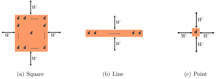
In this section, we will use three simple but practical 2-dimensional examples to give some intuition for the problem we are going to solve.
[image:13.612.125.497.497.633.2]d d d d …… …… d d d d d d d d d d …… …… d d d d W W W W …… …… ………… (a) Square d d d d … ……… d d d d W W (b) Line d d W W W W (c) Point
2.1.1
Example 1: All Demands Are in a Square
In this example, the demand is d at any point in a square T of size a×a and 0 at any point outside the square, which is shown in Figure 2.1(a).
Since the traveling cost between any two adjacent points is 1 unit of energy, only those vehicles within distance W could get into the area T. Therefore, W ×(2W + a)2 ≥ d×a2. Let W
1 be the solution to W ×(2W +a)2 = d×a2, where W is the
variable. ThenW ≥W1. When a approaches infinity, W approaches d.
2.1.2
Example 2: All Demands Are on a Line
In this example, the demand is d at any point on a line L and 0 at any other point, which is shown in Figure 2.1(b). It is a reasonable and practical model when using the mobile vehicles to detect the traffic flow on the highway.
Since the traveling cost between any two adjacent points is 1 unit of energy and only those vehicles within distanceW could get onto the lineL, we have W×(2W+ 1) ≥ d. Let W2 be the solution to W ×(2W + 1) = d, where W is the variable,
then W ≥ W2. If each vehicle has a capacity W = 2W2, there is a way to serve all
the demands: Any vehicle in the neighborhood of radius W2 around L, i.e. NW2(L), moves to its nearest point on the lineL. The traveling cost for each vehicle is at most
W2 units of energy and the remaining energy could be used to serve the demands.
This is shown in Figure 2.2. Therefore, W2 ∼d.
2.1.3
Example 3: All Demands Are in a Single Point
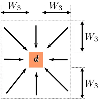
In this example, the demand is d at a single pointp and 0 at any other point, which is shown in Figure 2.1(c). It is a reasonable model when using the mobile vehicles to detect the earthquake.
Only those vehicles within distanceW could get intop. We haveW×(2W+1)2 ≥
d. Let W3 be the solution to W ×(2W + 1)2 = d, where W is the variable, then
W ≥ W3. If each vehicle has a capacity W = 3W3, there is a way to serve all the
d
d
d
d
…
………
……
d
d
d
d
… ………
… ………
W
2 [image:15.612.197.463.83.222.2]W
2Figure 2.2: Any vehicle in the neighborhood of radius W2 around the line L, i.e.
NW2(L), moves to its nearest point on the line.
at point p, moves to p. The traveling cost for each vehicle is at most 2W3 units of
[image:15.612.247.409.366.529.2]energy and the remaining energy is enough to serve the demands. This is shown in Figure 2.3. Therefore, W3 ∼d.
d
d
W
3W
3W
3W
3Figure 2.3: Any vehicle in the square of size (2W3+ 1)×(2W3+ 1), whose center is
at point p, moves to p.
2.2
Characterization of Optimal Off-line Performance
overhead. But we confine each vehicle to within a local neighborhood of a specified radius r >0 around its starting point. Later in the section, we will set the radius r
to be the same as the vehicle capacity.
The minimal capacity required for resolving the supply-demand transports with a specified radius parameter r is the solution of the following linear program (LP):
minimize ω
s.t.
P
j∈Nr(i)
fij ≤ω, ∀ i∈Z
ℓ
P
i∈Nr(j)
fij ≥d(j), ∀ j ∈Z
ℓ
fij ≥0, ∀ i, j ∈Z
ℓ
and ki−jk ≤r,
(2.1)
where F = {fij} denotes the set of “flows.” Each flow fij represents the amount of energy transported by the vehicle at position i to position j.
Notice that (2.1) is not the classical LP used in the classical “Transportation Problem” [15] in two important aspects:
• In the Transportation Problem, both the supply distribution (how much energy is in each vehicle) and demand distribution (how much energy is needed at each position) are known a priori. The goal is to find the minimal cost (i.e. the Earthmover Distance [15]) to transform one distribution into the other. In (2.1), the supply distribution is part of the linear program, which is to be solved. The method we use here is different from those methods used in the classical Transportation Problem.
• In the Transportation Problem, there is either no distance constraint or fixed distance constraint. In our case, the transport distance is bounded by a param-eter r and later by the supply (vehicle capacity), which is to be solved.
maximize P
j∈Zℓ
d(j)× min
i:ki−jk≤rαi
s.t. P
i∈Zℓ
αi ≤1,
αi ≥0, ∀ i∈Z
ℓ
(2.2)
is equivalent to
maximize P
j
d(j) P
T:Nr(j)⊆T h(T) s.t. P
T⊆Zℓ
h(T)|T| ≤1
h(T)≥0, ∀ T ⊆Zℓ
. (2.3)
where h denotes a mapping from the set of subsets of Zℓ to R.
Proof : We will prove the lemma by two steps:
1. The solution of (2.2) is at most the solution of (2.3).
For any (αi)i∈Zℓ that solves (2.2), we can define a mapping h from the set of
subsets of Zℓ toR, that is, for any T ⊆Zℓ,
h(T) =
max 0,min
i∈T αi−i∈N1max(T)\Tαi
if T is simply connected
0 otherwise
.
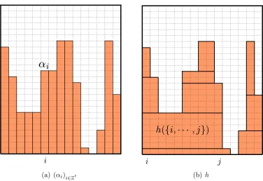
Given the value of(αi)i∈Zℓ as seen in Figure 2.4(a), h (in Figure 2.4(b)) can be
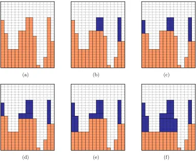
deduced by finding the maximalαi’s first and setting the value of those subsets to be the difference between the maximal value and the smaller value on the boundary; then reducing the value of (αi)i∈Zℓ on those subsets and repeating
the first step. Figure 2.5 gives an example of the first a few steps of the process.
Look at any two simply connected subsets T1, T2 of Z
ℓ
, which are related as follows:
i
i(a) (αi)i∈
Zℓ
j i
h
(
{i,
· · ·
, j}
)
[image:18.612.122.498.72.330.2](b) h
Figure 2.4: An illustration of the relationship between(αi)i∈Zℓ andhin 1-dimensional
space.
Suppose h(T1) 6= 0, i.e., min
i∈T1αi > i∈N1max(T1)\T1αi. Let x be a vertex in set T1 ∩
N1(T2)\T2 and y be a vertex in set T2∩N1(T1)\T1. Then
max
i∈N1(T2)\T2αi ≥αx ≥mini∈T1 αi ≥i∈N1max(T1)\T1αi ≥αy ≥mini∈T2 αi.
So h(T2) = 0. Therefore, for any two simply connected subsets T1, T2 of Z
ℓ
, if
h(T1)6= 0and h(T2)6= 0, then
T1 ⊂T2 or T1 ⊇T2 or T1∩T2 =∅.
For any i∈Zℓ
, there exist a sequence of sets T1, T2,· · · , Tκ such that
– i∈ T1 ⊂T2 ⊂ · · · ⊂Tκ ⊆Z
ℓ
,
– h(Tj)6= 0 for any j ∈ {1,2,· · · , κ},
(a) (b) (c)
[image:19.612.123.505.224.538.2](d) (e) (f)
From the definition of h, there exists an xj ∈Tj\Tj−1 for each j ∈ {2,3,· · · , κ}
such that
h(Tj) =
αi−αx2, j = 1
αxj−αxj+1, j ∈ {2,· · ·, κ−1}
αxκ, j =κ
.
Thus,
αi = κ
X
j=1
h(Tj) =
X
T:i∈T
h(T),
and
X
T⊆Zℓ
h(T)|T|= X
T⊆Zℓ
h(T)X
i:i∈T
1 = X
i:i∈Zℓ
X
T:i∈T
h(T) = X
i:i∈Zℓ
αi ≤1.
Given j ∈Zℓ, let x = arg min
i:ki−jk≤r
αi. For anyT such that x∈T and h(T) 6= 0, if
Nr(j) * T, then αx > αy for any y ∈ Nr(j)∩N1(T)\T, a contradiction with
αx = min
i:ki−jk≤rαi ≤αy. Therefore,
min
i:ki−jk≤rαi =
X
T:Nr(j)⊆T
h(T) for any j ∈Zℓ.
2. The solution of (2.3) is at most the solution of (2.2).
For any h that solves (2.3), we can define αi = P T:i∈T
h(T) for all i ∈ Zℓ. From
the definition, min
i:ki−jk≤rαi ≥
P
T:Nr(i)⊆T
h(T)for any j ∈Zℓ, and
X
i∈Zℓ
αi =
X
i∈Zℓ
X
T:i∈T
h(T) = X
T⊆Zℓ
h(T)X
i:i∈T
1 = X
T⊆Zℓ
h(T)|T| ≤1.
2
We are now ready to solve (2.1):
Lemma 2.2.2 Given d(x) ≥ 0 for all x ∈ Zℓ
and r > 0. The value of LP (2.1) is
max
T:T⊆Zℓ
Primal Dual
max
n
P
j=1
cjxj
s.t. Pn j=1
aijxj ≤bi (i= 1,· · · , m)
xj ≥0 (j = 1,· · · , n)
min
m
P
i=1
biyi
s.t. Pm i=1
aijyi ≥cj (j = 1,· · · , n)
yi ≥0 (i= 1,· · · , m)
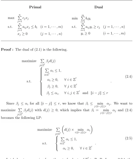
Proof : The dual of (2.1) is the following.
maximize P j∈Zℓ
βjd(j)
s.t. P
i∈Zℓ
αi ≤1,
αi ≥0, ∀ i∈Z
ℓ
βj ≥0, ∀ j ∈Z
ℓ
βj ≤αi, ∀ i, j ∈Z
ℓ
and ki−jk ≤r .
(2.4)
Since βj ≤ αi for all ki−jk ≤ r, we know that βi ≤ min
j:ki−jk≤rαj. We want to maximize P
j∈Zℓ
βjd(j) with d(j) ≥ 0, which implies that βi = min
j:ki−jk≤rαj and (2.4) becomes the following LP:
maximize P j∈Zℓ
d(j)× min
i:ki−jk≤rαi
s.t. P
i∈Zℓ
αi ≤1,
αi ≥0, ∀ i∈Z
ℓ .
(2.5)
[image:21.612.105.552.87.606.2]LP (2.5) is equivalent to
maximize P j
d(j) P
T:Nr(j)⊆T h(T) s.t. P
T⊆Zℓ
h(T)|T| ≤1
h(T)≥0, ∀T ⊆Zℓ
. (2.6)
Since P i
d(i) P
T:Nr(i)⊆T
h(T) = P
T⊆Zℓ
h(T) P
i:Nr(i)⊆T
d(i), the dual of (2.6) is
minimize ω
s.t. ω· |T| ≥ P i:Nr(i)⊆T
d(i), ∀ T ⊆Zℓ. (2.7)
Therefore, the solution of (2.1) is
ω= max
T:T⊆Zℓ
P
i:Nr(i)⊆T d(i)
|T| = maxT:T⊆Zℓ
P
x∈T
d(x)
|Nr(T)|
.
2
If we set the radius r to be ω, LP (2.1) becomes
minimize ω s.t. P
j∈Nω(i)
fij ≤ω, ∀i∈Z
ℓ
P
i∈Nω(j)
fij ≥d(j), ∀j ∈Z
ℓ
fij ≥0, ∀i, j ∈Z
ℓ
&ki−jk ≤ω
(2.8)
and the solution is as follows:
Lemma 2.2.3 Given d(x)≥0 for all x∈Zℓ
, the solution to program (2.8) is
max
T:T⊆Zℓ
ωT,
where ωT is the solution of ωT · |NωT(T)|=
P
T⊆Z
T1 = arg max
T⊆Zℓ
P
x∈T
d(x)
|Nr1(T)|
, and T2 = arg max
T⊆Zℓ
P
x∈T
d(x)
|Nr2(T)|
.
We see that ω(r)is a non-increasing function of r because
ω(r1)−ω(r2) = max
T⊆Zℓ
P
x∈T d(x) |Nr1(T)|
−max
T⊆Zℓ
P
x∈Td(x) |Nr2(T)|
=
P
x∈T1d(x) |Nr1(T1)|
−
P
x∈T2d(x) |Nr2(T2)|
≤
P
x∈T1d(x) |Nr1(T1)|
−
P
x∈T1d(x) |Nr2(T1)|
≤ 0.
Together with Lemma 2.2.2, the solution to program (2.8) is equal to the unique solution of the equation
ω= max
T⊆Zℓ
P
x∈T
d(x)
|Nω(T)|
, (2.9)
where ω is the variable. Let ω∗ be the solution of (2.8) and (2.9).
For any T′ ⊆Zℓ
,
ω∗ = max
T⊆Zℓ
P
x∈T
d(x)
|Nω∗(T)|
≥
P
x∈T′
d(x)
|Nω∗(T′)|
. (2.10)
Letω′ be the solution to the equation ω = P
x∈T′
d(x)
|Nω(T′)|. If ω
′ > ω∗, then
P
x∈T′
d(x)
|Nω∗(T′)|
≥
P
x∈T′
d(x)
|Nω′(T′)|
=ω′. (2.11)
Combining (2.10) with (2.11), we haveω∗ ≥ω′, a contradiction with the assumption.
Hence,ω∗ ≥ω′. Therefore, ω∗ = max
T:T⊆Zℓ
ωT, whereωT is the solution ofωT·|NωT(T)|=
P
x∈T d(x). 2
As used in the proof of Lemma 2.2.3, let ω∗ = max
T:T⊆Zℓ
account the cost of motion.
Corollary 2.2.4 Woff ≥ω∗= max T:T⊆Zℓ
ωT.
We are now ready for the upper bound on Woff.
Lemma 2.2.5 Woff ≤(2·3ℓ+ℓ)·ω∗ = (2·3ℓ+ℓ)· max T:T⊆Zℓ
ωT.
Remark: The primary interest in many applications is the plane (ℓ = 2). In the
plane, the upper bound is only a modest (and probably pessimistic) factor over the
lower bound. However, for generality, we perform the analysis for general ℓ.
Proof : In LP (2.8), for any position x ∈ Zℓ
, only those vehicles within distance ω
could move to x. According to Lemma 2.2.3, the amount of energy needed in any ⌈ω∗⌉ × ⌈ω∗⌉ × · · · × ⌈ω∗⌉
| {z }
ℓ
ℓ-cube is at mostω∗·(3⌈ω∗⌉)ℓ, excluding the travel overhead.
We partition the gridZℓ into⌈ω∗⌉×⌈ω∗⌉×· · ·×⌈ω∗⌉ℓ-cubes and provide each vehicle
with 2·3ℓ·ω∗ units of energy to serve customer demands. Thus, every vehicle only
needs to move and deliver energy inside its own ⌈ω∗⌉ × ⌈ω∗⌉ × · · · × ⌈ω∗⌉ ℓ-cube. In
every such ℓ-cube H, we have
X
x∈H
d(x)−3ℓ·ω∗ 3ℓ·ω∗
≤X
x∈H
d(x)
3ℓ·ω∗ ≤ ⌈ω ∗⌉ℓ
.
Let each vehicle use (leave) at most3ℓ·ω∗ energy first at its original position, and then
move to a particular position and serve the requests there. The traveling overhead for any vehicle is at most ℓ·ω∗. Therefore, at most (2·3ℓ+ℓ)·ω∗ energy is needed
for each vehicle. 2
Theorem 1.4.1 follows from Corollary 2.2.4 and Lemma 2.2.5. We also have the following two corollaries:
Corollary 2.2.6 Let Γ be the set of all ℓ-cubes in Zℓ
and ωT denote the solution of
ωT · |NωT(T)|=
P
x∈T d(x), then
max
T:T∈ΓωT ≤Woff ≤(2·3
max
T:T∈ΓωT ≤Tmax:T⊆ZℓωT ≤Woff.
Woff≤(2·3ℓ+ℓ)· max
T:T∈ΓωT follows as in the proof of Lemma 2.2.5. 2
Corollary 2.2.7 Let Γω be the set of all ⌈ω⌉ × ⌈ω⌉ × · · · × ⌈ω⌉ ℓ-cubes in Z
ℓ
. Define
ωc = min
ω:ω·(3⌈ω⌉)ℓ= max T∈Γω
P
x∈T d(x)
.
ωc ≤Woff ≤(2·3ℓ+ℓ)·ωc.
Proof : Assume that ωc is achieved when T =Tc. Then,
ωc·(3⌈ωc⌉)ℓ =
X
x∈Tc
d(x) =ωTc· |NωTc(Tc)|.
So we must haveωc ≤ωTc because otherwiseωc·(3⌈ωc⌉)
ℓ > ω
Tc·|NωTc(Tc)|. Therefore, ωc ≤ max
T:T⊆Zℓ
ωT and ωc ≤Woff. Finally, Woff ≤ (2·3ℓ+ℓ)·ωc follows as in the proof
of Lemma 2.2.5. 2
The characterization using cubes is much simpler than T ranging over all subsets of Zℓ. The fact that we only need to examine cubes in Zℓ is key to being able to provide an algorithm.
2.3
Approximation Algorithm to Compute
W
offFor simplicity, we shall restrict our analysis to 2-dimensions (ℓ = 2). The derivation for higher dimensions are straightforward extensions. We further assume that the graph is the n×n grid Zn×Zn where n is a power of 2 and the demand function is
d(x)≥0for every x∈Z2
n. Define
• The maximal demand is D= maxx∈Z2
nd(x).
• The average demand is Dˆ = P
x∈Z2nd(x)
Algorithm 1 Approximation algorithm to compute Woff, running in linear time
1 if n ≤Dˆ
2 return min{D, 2·Dˆ +ℓ·n};
3 if D ≤1
4 return D;
5 w←2, n′ ←n/w, d
1(i, j)←d(i, j);
6 if w=n
7 return min{D, 2·Dˆ +ℓ·n}; 8 for 1≤i≤n′,1≤j ≤n′
9 dw(i, j)←dw/2(2i−1,2j−1) +dw/2(2i−1,2j) +dw/2(2i,2j−1)
+dw/2(2i,2j);
10 if there exists a dw(i, j)> w·(3w)ℓ
11 w←2w, n′ ←n′/2;
12 goto 6;
13 else
14 return (2·3ℓ+ℓ)·w.
Notice that Woff has the following properties:
Property 2.3.1 Dˆ ≤Woff ≤D.
Proof : This is straightforward from the definition of Dˆ and D. 2
Property 2.3.2 If D≤1, then Woff =D.
Proof : From 2.3.1,Woff ≤D, soWoff ≤1, which means that the vehicles don’t have
enough energy to move. Therefore,Woff =D. 2
Property 2.3.3 If n≤Dˆ, then Woff ≤2·Dˆ +ℓ·n.
Proof : Since n ≤ Dˆ ≤ Woff, the whole grid does not need to be partitioned into small cubes and any vehicle can walk to any other point in the grid. The traveling overhead is upper bounded byℓ·n. Following the same reason as in Lemma 2.2.5, at most 2·Dˆ +ℓ·n energy is needed for each vehicle. 2
Using Corollary 2.2.7, together with Properties 2.3.1, 2.3.2, and 2.3.3, a2(2·3ℓ+ℓ) -approximation linear-time algorithm to compute Woff is given in Algorithm 1.
Analysis of Algorithm 1: Steps 1 to 5 will be visited only once and need time
O(nℓ); Steps 6 and 7 will be visited at mostlog
and need processing timeO(2ℓ)for each visiting; Steps 10 to 12 need processing time
O(nℓ
2ℓ + n ℓ
4ℓ +n ℓ
8ℓ +· · ·+ 1) =O( n ℓ
2ℓ−1). Therefore, the time complexity of Algorithm 1
is O(nℓ). In terms of memory requirement, each d
w is an ℓ-dimensional array of size
(n w)
Chapter 3
On-line case
In this chapter, we examine the on-line case of our Capacitated Multivehicle Routing Problem (CMVRP). In Section 3.1, we review the concept of diffusing computation, a technique used in our on-line algorithm. We give a decentralized on-line strategy for vehicles to serve jobs in Section 3.2. Finally, the characterization of optimal on-line performance (i.e. proof of Theorem 1.4.2) is provided in Section 3.3.
3.1
Diffusing Computations
In the seminal work [6], Dijkstra and Scholten first introduced the concept of diffusing computations in a distributed system of processes. A computation is diffusing when nodes receive information from another node (predecessor), and send it to all or a subset of their neighbors (successors). In such computations, a single active initial node awakens other nodes to perform some computation. These awoken nodes can spread the computation to other nodes, which then spread the computation further, and so on.
transition from idle to active status. The active node is always part of the tree. If a node that is already in the tree receives a request for activation, it notifies the sender that the tree’s topology need not change. A node can be removed from the tree by replying its parent when it is an idle leaf node (when replies have been received for all queries sent). Termination is detected when the tree contains only one idle node — the root node.
The algorithm assumes very little about the underlying graph which represents the network. Thus, it is suitable for application to a number of problems arising in distributed programming.
3.2
On-line Strategy
Unlike the off-line case where the demand distribution is known to all vehicles a priori, the on-line problem requires communication between the vehicles. Before proceeding further, we first state our assumptions about the communication model and the messaging protocol:
• The time interval between any two successive job arrivals is long enough to finish any computation and movement.
• This is a decentralized model: there is no central controller for the system.
• A vehicle can communicate with other vehicles by sending/receiving messages.
• When two vehicles are within a constant distance1
of each other, they are said to be neighbors. Neighbors can communicate directly with one another without having messages relayed through intermediate vehicles.
• The underlying communication topology is connected. That is, any two ve-hicles can communicate with each other by having messages go through some intermediate neighboring vehicles.
• The communication links are bidirectional.
• The communication cost is negligible: we assume communication requires no energy. If a vehicle uses up all its energy, it is still able to communicate with its neighbors and relay messages.
• A vehicle has only local knowledge: it knows the identities and positions of its neighbors; it is ignorant of the identities of all other vehicles and of the general structure of the network.
• Every vehicle has an input buffer of unbounded length. If vehicle P sends a message to a neighbor vehicle Q, then the message gets appended at the end of the input buffer of Q after a finite, arbitrary delay. The assumption of unbounded length buffers is for ease of exposition. It shall be apparent from
the strategy that the input buffer length of Q can be bounded by the number of
neighbors of Q.
• Error free communication: Messages are not lost or altered during transmission.
• Synchronous communication: Messages sent from P to Q arrive at Q’s input buffer in the order sent.
• Two messages arriving simultaneously at an input buffer are ordered arbitrarily and appended to the buffer. A process receives a message by removing one from its input buffer.
We further assume there is enough energy to follow the strategy and process all the jobs. In Section 3.3, we determine this required amount of energy for each vehicle.
As in Lemma 2.2.5, we partition Zℓ into ⌈ω
c⌉ × ⌈ωc⌉ × · · · × ⌈ωc⌉
| {z }
ℓ
ℓ-cubes (ωc is
defined in Corollary 2.2.7). The vertices of each cube are colored black or white according to:
Color(x) =
black if Pxi ≡0(mod 2)
If ⌈ωc⌉is even, the number of black vertices and the number of white vertices are equal. If ⌈ωc⌉ is odd, we assume (without loss of generality) there is 1 more black vertex in anyℓ-cube (if not, switch the colors of vertices in the cube). In this manner, each ℓ-cube can be further divided into pairs: each pair consists of two adjacent vertices: one black and one white; for odd ⌈ωc⌉, there may be a single black vertex left unpaired.
3.2.1
Vehicle State
We characterize the state of each vehicle by the pair: (S1, S2), where S1 represents
the working state of the vehicle and S2 represents the message-transfer state of the
vehicle.
The working state of the vehicle, S1, can be one of the following:
• Idle. Initially, all the vehicles at white vertices are idle. An idle vehicle does not serve any job but waits for a message to move to the specified vertex. After such move, the vehicle becomes active.
• Active. Initially, all the vehicles at black vertices areactive. An active vehicle will serve the jobs arriving at vertices that belong to the same pair as the vehicle belongs to. Because the two vertices belonging to the same pair are adjacent, the vehicle need walk at most distance 1.
• Done. When an active vehicle uses up its energy, its working state becomes
done.
The message-transfer state of the vehicle, S2, can be one of the following:
• Initiator. When an active vehicle becomes done, there is no vehicle to serve the jobs arriving at the vertices in the same pair. A replacing candidate — an
idle vehicle in the sameℓ-cube — needs to be found and sent a message with the
candidateidlevehicle. (In a centralized system, the candidateidle vehicle could be easily found and messaged.) Thedone vehicle starts a new computation and is the initiator of the diffusing computation.
• Waiting. Initially, all the vehicles arewaiting for signals to partake in a diffus-ing computation. When the computation finishes, vehicles change back to the
waiting state.
• Searching. When awaiting vehicle receives a signal of a diffusing computation, its state changes tosearching. When it has finished all its computation, its state returns to waiting again.
The state transition diagram is shown in Figure 3.1. Since an active or idle vehicle can not be the initiator of a diffusing computation, the states (active, initiator) and (idle,initiator) are not valid states.
idle, waiting active, waiting done, waiting
idle, searching active, searching done, searching
done, initiator
? 6 ? 6 ? 6
[image:32.612.116.535.378.445.2]
-XXXz :
Figure 3.1: State Transition Diagram. States (active, initiator) and (idle, initiator) are not valid states.
3.2.2
The Overall Structure
Our scheme has two parts. The first part is the processing of the jobs. When a job arrives at a vertex, if there is an active vehicle at the vertex, then it serves the job; if not, there must be an active vehicle at the other vertex in the same pair and that vehicle will serve the job.
candidate will have been identified. In phase II, a message will be transmitted along the path, which is identified in phase I, from the done vehicle to the candidate. Upon receiving the message, the candidate will move to the position of the done vehicle and become active.
In the remainder of the section, we focus on the algorithm for finding a candidate by diffusing computation and the algorithm for replacing the done vehicle.
3.2.3
Phase I Computation
3.2.3.1 Messages Used in Phase I
Phase I computation uses two kinds of messages:
• Aquery message associated with the pair (init, p), whereinitis the initiator of the computation andpis the identity of the vehicle sending the message. vehicle
p sends a query message to all its neighbors in the same ℓ-cube. Intuitively, a
query message signals that the vehicle is asking its neighbors if they are idle vehicles.
• A reply message to a query is a pair (f lag, p), where p is the identity of the vehicle sending the message and f lag is a boolean value. A vehicle p sends a
reply message to vehicleq in response to a query message sent byq. Intuitively, areply message withflag=true denotes thatphas found anidle vehicle; areply
message withflag=false denotes that p has not found an idle vehicle.
3.2.3.2 Local Data Used By a Vehicle During Phase I
num This is the number of un-responded messages, that is, the number of messages sent by this vehicle for which no reply message has been received so far.
child The successor (child) identity from which the firstreply message withflag=true
was received.
init This is the initiator identity of the diffusing computation. Initially it is NULL. It is used to distinguish diffusing computations initiated by different vehicles and to avoid joining the same computation more than once. If we tag the diffusing computation with another sequence numberk, we can also keep track of diffusing computations initiated at different times by the same vertex.
3.2.3.3 Phase I Algorithm Description
• When anactive vehicle becomesdone, its status changes from (active,waiting) to (done, initiator). It sends out a query message to all its neighbors. Its par
is NULL. When it receives the first reply message with flag=true, it sets child
to be the sender of the message. When all its messages have been responded,
i.e. num=0, the vehicle changes its status to (done, waiting).
• When awaiting vehicle receives aquery message with aninitdifferent from its current initiator identity, it records the sender of the query as its par, updates its init to be the init associated with the query. If it is an idle vehicle, send back a reply message with flag=true. If it is not an idle vehicle, change its status to searching, and sendquery messages to all its neighbors.
• When a non-waiting vehicle receives a query message, or a waiting vehicle re-ceives a query message with an init same as its current initiator identity, send back a reply message with flag=false immediately.
• When a searching vehicle receives the firstreply message withflag=true, set its
child to be the sender of the message and send a reply message with flag=true
to its par.
• When a searching vehicle has received replies from each of its neighbors, i.e. num=0, it changes status to waiting. If itschild is NULL, it sends areply with
has finished and a path to a candidate idle vehicle has been established. The details of the algorithm in Phase I are given in Algorithms 2.
3.2.4
Phase II Computation
Phase II employs only one kind of message: Move along with the destination asso-ciated with it. When the initiator of the diffusing computation changes its status to
waiting, the computation has been finished. Initiator p sends out amove(location of
p) message to its child, itschild copies it to the next child, and the process continues until we reach an idle vehicle. The idle vehicle then moves to the location of p and changes its state to (active, waiting).
3.2.5
Discussion
In the previous sections, we have described a decentralized on-line strategy for vehicles to serve jobs. The strategy works under the condition that all the vehicles work well. But in practice, a done vehicle could fail to initialize a diffusing computation, an
active vehicle could break down and become dead (it can’t process jobs any more). We distinguish among these four different scenarios:
1. All the vehicles work well and no exception occurs.
2. There are done vehicles failing to initialize a diffusing computation, but no vehicles breaking down and becoming dead.
3. There are constant number ofactive vehicles breaking down and becomingdead.
4. There are large (more than constant) number of active vehicles breaking down and becoming dead.
Algorithm 2 Phase I Algorithm.
When a vehicle p uses up its energy:
1. p.s1 ← done,p.s2 ← initiator;
2. p.par ← NULL; 3. p.init ←p;
4. send query(p, p) to all its neighbors; 5. p.num ← the number of neighbors of p.
For a vehicle p upon receiving an query message (init, q):
1. If p.s2 = waiting & p.init 6=init
2. p.par ←q; 3. p.init ←init; 4. p.child ←NULL; 5. Ifp.s1 = idle
6. send areply message (true,p) to q; 7. else
8. p.s2 ← searching;
9. send query messages (init, p) to all its neighbors; 10. p.num ← the number of neighbors of p;
11. else
12. send a reply message (false,p) to q.
For a vehicle p upon receiving an reply message (flag, q):
1. p.num ← p.num - 1;
2. If flag=true and this is the first reply message with flag=true it receives 3. p.child ←q;
4. send a reply message (true, p) to p.par; 5. If p.num=0
6. p.s2 ← waiting;
7. Ifp.child=NULL
which points to one of its active neighbors. Any active vehicle is pointed by a unique “monitoring” pointer. All the pointers form a loop.
A vehicle sends out “existing” messages periodically to notify its neighbors that it is still there. If a vehicle has not received the “existing” messages from the neighbor its “monitoring” pointer pointing to for a certain time, it decides that the neighbor is
done and initializes a diffusing computation for the neighbor. The replacing vehicle for the done vehicle needs to update its “monitoring” pointer to maintain the loop.
When the misfortune of scenario 3 occurs, since there are only constant number of active vehicles breaking down and the overall energy requirement changes very slightly, the energy constraint is not a concern. We can use the same way used in the second scenario to initialize a diffusing computation.
The scenario 4 is different from the other scenarios, which will be discussed in Chapter 4.
3.3
Proof of Theorem 1.4.2
Lemma 3.3.1 Won ≤(4·3ℓ+ℓ)·ωc = (4·3ℓ+ℓ)· max T:T⊆Zℓ
ωT, where ωT denotes the
solution of the equation ωT · |NωT(T)|=
P
x∈T d(x).
Proof : In order to satisfy the requirement that upon a job arrival, there exists an
active vehicle in each black-white pair, we need to make sure that after all jobs have arrived, there still exists an active vehicle in each black-white pair. According to Corollary 2.2.7, the amount of energy needed in any ⌈ωc⌉ × ⌈ωc⌉ × · · · × ⌈ωc⌉
| {z }
ℓ
ℓ-cube
is at most ωc(3⌈ωc⌉)ℓ, excluding the travel overhead. Since the processing of each job requires a walk of distance at most 1, at most 2·ωc(3⌈ωc⌉)ℓ units of energy is needed in each cube for job processing. If each vehicle is given 4·3ℓ·ω
c units of energy for processing jobs, then after all jobs have arrived and been processed, there are at least
4·3ℓ·ω
c· ⌈ωc⌉ℓ−2·ωc(3⌈ωc⌉)ℓ
4·3ℓ·ω c
= ⌈ωc⌉
ℓ
vehicles with energy left, which means there exists an active vehicle in each black-white pair. The distance between any two vertices in the same cube in at mostℓ·ωc, which implies that an idle vehicle needs to move a distance at mostℓ·ωc to become
active. Therefore, at most (4·3ℓ+ℓ)·ω
c units of energy is needed for each vehicle for the on-line case. Since ωc ≤ max
T:T⊆Zℓ
ωT (see in the proof of Corollary 2.2.7), the
lemma is proven. 2
Clearly, Won ≥Woff ≥ max
T:T⊆Zℓ
ωT, whereωT denotes the solution ofωT· |NωT(T)|=
P
Chapter 4
Different Case Study: Broken
Vehicles
In Chapter 2, we discussed the problem of minimizing the initial energy needed for each vehicle in the off-line case and showed that Woff is of the same order as the solution to program (2.8), which is
Woff= Θ
max
T:T⊆Zℓ
ωT
,
whereωT is the solution of ωT· |NωT(T)|=
P
x∈T d(x). Furthermore, we showed that
Won is of the same order as Woff in Chapter 3.
We now extend the problem to allow a large number of vehicles breaking down, which is the fourth scenario mentioned in Section 3.2.5.
For each vehicle i there is a “longevity” parameter pi(0≤ pi ≤ 1). The vehicle i breaks at the time when a fraction pi of its initial energy has been used. If pi = 0, the vehicle breaks initially; if pi = 1, the vehicle will not break.
In the off-line case, the demand functiond(·), arrival sequence, and the “longevity” parameters are known at the beginning. LetWoff-b denote the minimal W needed in the off-line case when a large number of vehicles breaking down is allowed.
4.1
Lower Bound on
W
off-bIn this section, we use the same method as in Section 2.2 to get a lower bound on
Woff-b.
Theorem 4.1.1 Woff-b ≥ max T:T⊆Zℓ
ωT, where ωT is the solution of ωT · P i∈Npi·ωT(T)
pi =
P
i∈T
d(i). 2
Proof : Straightforwardly, the solution to the following programming (4.1) is a lower bound onWoff-b.
minimize ω s.t. P
j∈Npi·ω(i)
fij ≤pi·ω, ∀ i∈Z
ℓ
P
i∈Npi·ω(j)
fij ≥d(j), ∀ j ∈ Z
ℓ
fij ≥0, ∀ i, j ∈Z
ℓ
& ki−jk ≤pi·ω,
(4.1)
where F = {fij} denotes the set of “flows.” Each flow fij represents the amount of energy transported by the vehicle at position i to position j.
Since we are using the same method as in Section 2.2 to solve (4.1), we will just give an outline of the proof in the following.
We first study the following linear program (LP):
minimize ω s.t. P
j∈Npi·r(i)
fij ≤pi·ω, ∀ i∈Z
ℓ
P
i∈Npi·r(j)
fij ≥d(j), ∀ j ∈Z
ℓ
fij ≥0, ∀ i, j ∈Z
ℓ
and ki−jk ≤pi·r
maximize P j∈Zℓ
βjd(j)
s.t. P
i∈Zℓ
pi·αi ≤1,
αi ≥0, ∀ i∈Z
ℓ
βj ≥0, ∀ j ∈Z
ℓ
βj ≤αi, ∀ i, j ∈Z
ℓ
and ki−jk ≤pi·r
(4.3)
which simplifies to the LP:
maximize P j∈Zℓ
d(j)× min
i:ki−jk≤pi·rαi
s.t. P
i∈Zℓ
pi·αi ≤1,
αi ≥0, ∀i∈Z
ℓ
(4.4)
Lethdenote a mapping from the set of subsets ofZℓ toR, then (4.4) is equivalent to
maximize P j
d(j) P
T:{i:ki−jk≤pi·r}⊆T
h(T) ! s.t. P
T⊆Zℓ
h(T)P
i∈T
pi
≤1
h(T)≥0, ∀ T ⊆ Zℓ
(4.5)
The dual of (4.5) is
minimize ω
s.t. ω· P i∈T
pi ≥ P
j:{i:ki−jk≤pi·r}⊆T
d(j), ∀ T ⊆Zℓ (4.6)
Therefore, the solution of (4.2) is
ω = max
T:T⊆Zℓ
P
j:{i:ki−jk≤pi·r}⊆T
d(j)
P
i∈T
pi
= max
T:T⊆Zℓ
P
i∈T
d(i)
P
i∈Npi·r(T) pi
Let ω(r) = max
T:T⊆Zℓ
i∈T
d(i)
P
i∈Npi·r(T)
pi. We see that ω(r) is a non-increasing function of r. Therefore, the solution to the program (4.1) is the same as the solution of the equation r=ω(r), which is max
T:T⊆Zℓ
ωT. 2
4.2
An Example of a Large
W
off-bIn this section, we use an example to illustrate the difference between Woff-b and the
solution to (4.1).
i k j
[image:42.612.180.470.260.485.2]r2
r1
r1
r2
Figure 4.1: A scenario illustration. Every vehiclex outside the circle (green position) has px = 1; the vehicle at k (green point in the circle) has pk = 1; any other vehicle
x has px = 0. The demands at i and j (red points) are d(i) =d(j) = r1; the demand
at any other position is 0.
Consider the scenario shown in Figure 4.1. The distance between i and k is
D(i, k) =r1. The distance between j and k is also D(j, k) = r1. D(i, j) = 2r1. The
distance fromi orj to the boundary of the circle isr2 ≫r1. Every vehicle xoutside
the circle has px = 1; the vehicle at the green position k in the circle has pk = 1; other vehicles have px = 0. The demands atiand j (red points) ared(i) =d(j) =r1;
the demand at any other position is 0. The service requests arrive at positions i and
is achieved when fki =r1, fkj =r1.
Assume Woff-b is of order r1. Since r2 ≫ r1, the non-broken vehicles outside the
circle can’t move to positionsiorj. The only remaining non-broken vehicle is k. The vehicle k needs to walk back and forth between i and j because the service requests arrive at positions i and j alternatively. In order to serve all the requests, the travel distance ofkisr1+(2r1−1)·2r1, which is not of orderr1. A contradiction. Therefore,
Woff-b is not of order r1 and Woff-b=ω(r1).
Chapter 5
Inter-Vehicle Energy Transfers
In Chapters 2 and 3, we discussed the problem of minimizing the initial energy needed for each vehicle in the off-line and on-line cases respectively. We now extend the problem to allow inter-vehicle energy transfers. That is, vehicleAcan transfer energy to vehicle B when A and B are at the same location. We consider two methods of accounting for energy transfers:
• Fixed cost: Chargea1 units of energy per transfer, no matter how much energy
is transferred, or
• Variable cost: Charge a2 ≪1units of energy per unit of energy transferred.
It turns out that, no matter which accounting method is used, under the same job load, the minimal vehicle capacity W needed with energy transfer allowed is of the same order as that without energy transfer. We let Wtrans-off andWtrans-on denote
the minimalW in the off-line and on-line energy-transfer cases respectively. Clearly,
Wtrans-off ≤Wtrans-on, Wtrans-off ≤Woff, and Wtrans-on ≤Won,
In this section, the analysis in the proof of Theorem 5.1.1 gives a lower bound on
Wtrans-off. It works for both energy-transfer accounting methods: the fixed cost sce-nario where each transfer costs a1 units regardless of amount transferred, and the
variable cost scenario where the transfer costs a2 units per unit of energy transferred.
Once again, for simplicity, we only study the two-dimensional (ℓ= 2) case.
Theorem 5.1.1 Wtrans-off = Θ(Woff).
Proof : Since there is at mostWtrans-off units of energy in each vehicle, the minimum traveling cost per unit energy per distance is 1
Wtrans-off
1
. Moving Wtrans-off units of energy from a position i to another position j will cost energy at least
Wtrans-off× 1
Wtrans-off +Wtrans-off
1− 1
Wtrans-off
× 1
Wtrans-off
+· · ·+Wtrans-off
1− 1
Wtrans-off
ki−jk−1
× 1
Wtrans-off
= Wtrans-off× 1−
1− 1
Wtrans-off
ki−jk! ,
and so the left energy amount is at most Wtrans-off ×1− 1
Wtrans-off
ki−jk
, no matter how many transfers of energy occur, nor which transfer accounting method is used.
Therefore, when moving Wtrans-off units of energy from position i into an s ×s
square T ⊆Z2, the amount of remaining energy, which is initially fromi, is at most
Wtrans-off×
1− 1
Wtrans-off
D(i,T)
,
where D(i, T) is the Manhattan distance from the point i to the squareT. The amount of energy initially in the square T isWtrans-off×s2. Since
|{i:D(i, T) =r}|= 4s+ 4(r−1),
the total amount of energy that can be moved into the square T is at most
Wtrans-off×s2+ ∞
X
r=1
Wtrans-off×(1− 1
Wtrans-off)
r×(4s+ 4(r−1))
= Wtrans-off× s2+ 4 ∞
X
r=1
(1− 1
Wtrans-off
)r×(r+s−1)
!
= Wtrans-off× s2+ 4 ∞
X
r=1
r(1− 1
Wtrans-off)
r+ 4(s−1)
∞
X
r=1
(1− 1
Wtrans-off)
r
!
= Wtrans-off× s2+ 4(Wtrans-off−1)Wtrans-off+ 4(s−1)(Wtrans-off−1)
= Wtrans-off× s2+ 4Wtrans-off2 + 4sWtrans-off−8Wtrans-off−4s+ 4
,
which should be at least the total demand in T. That is,
Wtrans-off× s2+ 4Wtrans-off2 + 4sWtrans-off−8Wtrans-off−4s+ 4
≥X
i∈T
d(i).
Since
|NWtrans-off(T)|
= Θ s2+Wtrans-off2
= Θ s2+ 4Wtrans-off2 + 4sWtrans-off−8Wtrans-off −4s+ 4
,
we have that Wtrans-off = Ω (ωT), where ωT denotes the solution of ωT · |NωT(T)| =
P
x∈T d(x). Let Γ be the set of all squares in Z2. ThenWtrans-off = Ω
max
T∈ΓωT
.
By Corollary 2.2.6, Woff = Θ
max
T∈Γ ωT
. Since Wtrans-off ≤ Woff, we have that
Wtrans-off = Θ
max
T∈Γ ωT
= Θ(Woff). 2
Corollary 5.1.2 Wtrans-off, Wtrans-on, Woff, and Won are Θ
max
T ωT
Often in practical applications, the vehicle tanks might not be full initially. Let W
denote the initial energy andC > W denote the vehicle tank capacity. When energy transfer is not allowed, the minimal W is the same as discussed in Chapters 2 and 3 regardless of C. However, when energy transfer is allowed, large capacity tanks can improve performance. We present an interesting example where Wtrans−off =
Θ (avgxd(x)).
5.2.1
An example of
Wtrans−off
with
C
=
∞
For this illustration, one dimension suffices. Consider a line segment of length N
(vertices numbered 1 through N). When the vehicle capacities are infinite, we let vehicle-1 travel toN while collecting energy from vehicles2,3, . . . , N−1along the way. AtN, it exchanges energy with vehicleN such that vehicle-N has exactly the amount of energy required to process the jobs at its position. After the exchange, vehicle-1 walks back to its original position while distributing energy to vehicles N−1, . . . ,3,2
according to the demand required at each position. In total, the number of energy transfers is2N −3 and the distance traveled is 2N −2.
• In the fixed cost scenario where each transfer costsa1 units regardless of amount
transferred, the total energy needed is
Etotal=a1·(2N −3) + (2N −2) +
X
x
d(x).
Then
Wtrans−off =
a1 ·(2N −3) + (2N −2) +Pxd(x)
N
= 2a1 + 2 +
P
xd(x)−3a1−2
N .
transferred, the total energy needed is
Etotal =a2·Wtrans−off·(2N−3) + (2N −2) +
X
x
d(x).
Then
Wtrans−off ·N =a2·Wtrans−off·(2N−3) + (2N −2) +
X
x
d(x)
⇒ Wtrans−off =
2N −2 +Pxd(x) N −2a2N + 3a2
.
Therefore, Wtrans−off = Θ (Pxd(x)/N) = Θ (avgxd(x)), no matter which
energy-transfer accounting method is used.
Chapter 6
Conclusions and Future Works
The key concepts/contributions of the thesis is as follows:
• The minimal energy needed in the off-line case is of the same order as that of the on-line case.
• We proposed an algorithm and a strategy for the Capacitated Multivehicle Routing Problem.
We note that the proposed algorithm represents only an initial prototype. We expect that this thesis will provide an incentive for future work on this problem. There are also several immediate research directions that can be pursued:
• The example from Section 5.2.1 shows that when inter-vehicle energy transfer is allowed and vehicles posses (non-full) large-capacity tanks, there can be sig-nificant energy savings. The questions of how much energy could be saved in general remains open.
• One can explore further the precise relationship between Woff and Won, trying
to tighten the constant factor, which is exponential inℓ. In particular, it would be nice to show that the exponential dependence on ℓ is unnecessary.
Bibliography
[1] L. Bodin and B. Golden. Classification in vehicle routing and scheduling. Net-works, 11(2):97–108, 1981.
[2] J. Bramel and D. Simchi-Levi. Probabilistic analyses and practical algorithms for the vehicle routing problem with time windows. Operations Research, 44(3):501– 509, 1996.
[3] O. Bräysy and M. Gendreau. Vehicle routing problem with time windows, part i: Route construction and local search algorithms. Transportation Science, 39(1):104–118, 2005.
[4] G. Clarke and J. W. Wright. Scheduling of vehicles from a central depot to a number of delivery points. Operations Research, 12(4):568–581, 1964.
[5] G. B. Dantzig and J. H. Ramser. The truck dispatching problem. Management Science, 6(1):80–91, 1959.
[6] E. W. Dijkstra and C. S. Scholten. Termination detection for diffusing compu-tations. Inf. Proc. Letters, 11(1):1–4, 1980.
[7] M. L. Fisher. Optimal solution of vehicle routing problems using minimum k-trees. Operations Research, 42(4):626–642, 1994.
[9] B. E. Gillet and L. R. Miller. A heuristic algorithm for the vehicle - dispatch problem. Operations Research, 22(2):340–349, 1974.
[10] J. M. Kahn, R. H. Katz, and K. S. J. Pister. Next century challenges: Mobile networking for “smart dust”. In International Conference on Mobile Computing and Networking (MOBICOM), pages 271–278, 1999.
[11] N. Katoh and T. Yano. An approximation algorithm for the pickup and delivery vehicle routing problem on trees. Discrete Appl. Math., 154(16):2335–2349, 2006.
[12] G. Laporte. The vehicle routing problem: An overview of exact and approximate algorithms. European J. Oper. Res., 59:345–358, 1992.
[13] T. Ralphs, J. Hartman, and M. Galati. Capacitated vehicle routing and some related problems. Some CVRP Slides, Rutgers University, 2001.
[14] T. Ralphs, L. Kopman, W. Pulleyblank, and L. Trotter. On the capacitated vehicle routing problem. Accepted to Mathematical Programming, 2001.
[15] Y. Rubner, C. Tomasi, and L. J. Guibas. The earth mover’s distance as a metric for image retrieval. Int. J. Comput. Vision, 40(2):99–121, 2000.
[16] M. M. Solomon. Algorithms for the vehicle routing problem with time windows.
Transportation Science, 29(2):156–166, 1995.
[17] P. Toth and D. Vigo. An overview of vehicle routing problems. pages 1–26, 2001.
[18] B. Warneke, M. Last, B. Liebowitz, and K. S. J. Pister. Smart dust: Communi-cating with a cubic-millimeter computer. Computer, 34(1):44–51, 2001.
[19] A. Wren. Computers in transport planning and operation. Operational Research Quarterly, 23(3):404–405, 1972.