Transfer function optimization for volume visualization based on visibility and saliency

Transfer Function Optimization for Volume

Visualization Based on Visibility and Saliency

by

Shengzhou Luo

Dissertation

Presented to the

University of Dublin, Trinity College

in fulfillment

of the requirements

for the Degree of

Doctor of Philosophy

University of Dublin, Trinity College

Declaration

I, the undersigned, declare that this work has not previously been submitted as an

exercise for a degree at this, or any other University, and that unless otherwise stated,

is my own work.

Shengzhou Luo

Permission to Lend and/or Copy

I, the undersigned, agree that Trinity College Library may lend or copy this thesis

upon request.

Shengzhou Luo

Acknowledgments

I wish to express my sincerest thanks and gratitude to my supervisor Dr John Dingliana,

for all his help, encouragement and support. This work would not have been possible

without him.

Thanks are also due to my friends and colleagues in the Graphics Vision and

Visual-isation group (GV2), past and present, for making my time there thoroughly enjoyable

and memorable. I also wish to acknowledge the contribution of Tom Noonan. His

collaboration on GPU-based visibility computation was a great help to my work.

Finally, I would like to especially thank my parents, my sister and Lu Han, to whom

I am forever indebted for their support, encouragement and patience throughout this

research.

Shengzhou Luo

Transfer Function Optimization for Volume

Visualization Based on Visibility and Saliency

Publication No.

Shengzhou Luo, Ph.D.

University of Dublin, Trinity College, 2016

Supervisor: John Dingliana

Volume data is widely used in scientific and medical research, and volume

visu-alization techniques aim to provide effective and flexible methods for analyzing and

exploring complex structures in such data. However, obtaining clear visualization of

features of interest in volume data is still a major challenge. One time-consuming and

unitintuitive part of the process is the specification of an appropriate transfer function,

which determines the classification and visibility of features. In practice, this is

typi-cally achieved using a trial-and-error approach: modifications are made to the transfer

function and changes in the resulting visualization are carefully observed in order to

This thesis proposes and investigates novel automated optimization techniques for

transfer functions, in order to emphasize features of interest. These techniques exploit

information content associated with volume data and objective measures based on

visual saliency and visibility in volume visualization.

We describe a global optimization and two user-driven refinement methods for

mod-ulating transfer functions in order to assist the exploration of volume data. This

op-timization is dependent on the distribution of the scalar values of the volume data

set and is designed to reduce general occlusion and improve the clarity of layers of

structures in the resulting images.

In addition to view-independent information, we propose a novel view-dependent

measure called visibility-weighted saliency in order to assist users in choosing suitable

viewpoints and designing effective transfer functions to visualize the features of interest

in a volume rendered images. This measure is based on a computational measure of

perceptual importance of voxels and the visibility of features in volume rendered images.

Subsequently, we present an automated transfer function optimization method

based on the visibility-weighted saliency metric. This method takes into account the

perceptual importance of voxels and the visibility of features, and automatically

ad-justs the transfer function to match the target saliency levels specified by the user. In

addition, a parallel line search strategy is presented to improve the performance of the

optimization algorithm.

Finally, we describe a multivariate visualization approach which modulates focus,

emphasizing important information, by adjusting saturation and brightness of voxels

Contents

Acknowledgments vii

Abstract ix

List of Tables xv

List of Figures xvii

Chapter 1 Introduction 1

1.1 Motivation . . . 2

1.2 Scope . . . 2

1.3 Contributions . . . 3

1.4 Summary of Chapters . . . 4

Chapter 2 Related Work 7 2.1 Volume Rendering . . . 7

2.1.1 Volume Ray Casting . . . 9

2.1.2 Splatting . . . 9

2.1.3 Shear Warp . . . 10

2.1.4 Texture-Based Volume Rendering . . . 10

2.1.5 Illustrative Volume Visualization . . . 11

2.2 Transfer Functions . . . 12

2.3 Automated Transfer Function Generation . . . 16

2.4 Visibility Histograms and Visibility-Driven Transfer Functions . . . 17

2.5 Multivariate Volume Visualization . . . 21

2.6.1 Transfer Functions for Time-Varying Volume Visualization . . . 22

2.6.2 Visualizing Time-Varying Volume Data with Non-Photorealistic Rendering . . . 25

2.6.3 Vector Field Visualization . . . 26

2.6.4 Feature Tracking . . . 26

2.7 Information Theory in Visualization . . . 28

2.8 Computational Saliency in Visualization . . . 29

2.9 Perceptual Evaluation . . . 30

2.10 Summary . . . 31

Chapter 3 Information-Guided Transfer Function Refinement for Ex-ploring Volume Data 33 3.1 Introduction . . . 33

3.2 Related Work . . . 34

3.3 Background . . . 35

3.3.1 Transfer Function Specification . . . 35

3.3.2 Entropy of Volume Data . . . 37

3.4 Method . . . 38

3.4.1 Weighting of Transfer Function Components . . . 38

3.4.2 Optimizer . . . 39

3.4.3 Prioritizing Intensity Ranges . . . 41

3.4.4 Adaptive Transfer Functions for Time-Varying Data Sets . . . . 44

3.5 Results and Discussions . . . 44

3.5.1 Automatic Transfer Function Refinement . . . 46

3.5.2 Transfer Function Refinement with User-Selected Intensity Values 49 3.5.3 Transfer Function Refinement with User-Selected Regions . . . 49

3.5.4 Adaptive Transfer Functions for Time-Varying Data Sets . . . . 49

3.6 Conclusions . . . 52

Chapter 4 Visibility-Weighted Saliency for Volume Visualization 55 4.1 Introduction . . . 55

4.2 Related Work . . . 56

4.3.1 Feature Definition . . . 58

4.3.2 Visibility Fields . . . 58

4.3.3 Saliency Fields . . . 61

4.3.4 Visibility-Weighted Saliency Fields of Features . . . 62

4.3.5 Visibility-Weighted Saliency (VWS) Histograms . . . 64

4.4 Use Case: Measuring Feature Saliency Resulting from Different Transfer Functions . . . 68

4.5 Experiment . . . 68

4.5.1 Source Images and Participants . . . 72

4.5.2 Methods and Measurements . . . 73

4.5.3 2D Feature Saliency (2DFS) . . . 73

4.5.4 Feature Visibility (FV) . . . 74

4.5.5 Data Analysis . . . 74

4.5.6 Varying Saturation and Brightness in Transfer Functions . . . . 77

4.6 Conclusions . . . 79

Chapter 5 Transfer Function Optimization Using Visibility-Weighted Saliency 81 5.1 Introduction . . . 81

5.2 Related Work . . . 82

5.3 Method . . . 83

5.3.1 Objective Function . . . 83

5.3.2 Parameter Space . . . 85

5.3.3 Optimization Algorithm . . . 86

5.3.4 Estimating Descent Directions . . . 88

5.3.5 Line Search and Parallel Line Search . . . 90

5.4 Results and Discussions . . . 94

5.4.1 Transfer Function Optimization For Time-Varying Data Sets . . 102

5.4.2 Generality of Transfer Functions . . . 103

5.5 Conclusions . . . 108

Chapter 6 Selective Saturation and Brightness for Visualizing

6.1 Introduction . . . 109

6.2 Related Work . . . 110

6.3 Method . . . 110

6.4 Results . . . 111

6.5 Conclusions . . . 116

Chapter 7 Conclusions 117 7.1 Summary of Contributions . . . 117

7.2 Limitations and Future Work . . . 118

7.2.1 Automated Transfer Function Approaches . . . 118

7.2.2 Visibility-Weighted Saliency . . . 119

7.2.3 Selective Saturation and Brightness . . . 120

Appendix A Estimating Feature Saliency Using 2D Saliency Maps 121

Appendix B Experiment Questionnaire 127

List of Tables

3.1 Hounsfield units of some typical substances [1] . . . 35 3.2 Computation time (seconds) for optimizations . . . 40

List of Figures

2.1 Voxels (cubic elements) constituting a volume data set [2]. . . 8

2.2 A sliced image of the data set . . . 8

2.3 Volume rendering of the data set . . . 8

2.4 The VisMale data set [3] . . . 8

2.5 Slight changes in the transfer function causes significant difference in the resulting images [4] . . . 12

2.6 Visibility histograms [5] . . . 19

2.7 Opacities and feature visibilities of 4 features highlighted in different colors [6] . . . 20

2.8 A single static transfer function cannot capture dynamic features. . . . 24

3.1 Typical transfer function shapes [7] . . . 36

3.2 A transfer function with tent-like shapes . . . 36

3.3 A screenshot of our volume rendering system . . . 45

3.4 Before optimization: CT-Knee with a continuous transfer function . . . 47

3.5 After optimization: CT-Knee with the continuous transfer function . . 47

3.6 Before optimization: CT-Knee with a transfer function of tent-like shapes 48 3.7 After optimization: CT-Knee rendered with the transfer function of tent-like shapes . . . 48

3.8 The 3 chosen colors and the transfer functions after optimization . . . . 50

3.14 Histograms and transfer functions for time-steps 0 and 50 respectively . 54

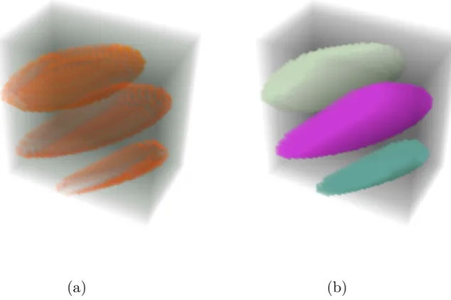
4.1 A synthetic volume data set consisting of three solid disk-like features . 60

4.2 The saliency fields computed from brightness and saturation respectively 62

4.3 The saliency fields emphasize the center and de-emphasize the surround-ings of voxels. . . 63

4.4 Visibility-weighted saliency fields of the three disks . . . 65

4.5 The feature visibility histogram and the visibility-weighted saliency his-tograms from the left viewpoint . . . 66

4.6 The feature visibility histogram and the visibility-weighted saliency his-tograms from the right viewpoint . . . 67

4.7 A tooth data set with a transfer function revealing three features . . . 69

4.8 Visibility-weighted saliency fields of the three features . . . 69

4.9 Feature visibility and visibility-weighted saliency of the three features . 70

4.10 A tooth data set with a transfer function particularly highlighting the enamel (the yellow feature) . . . 70

4.11 Visibility-weighted saliency field of the three features . . . 71

4.12 Feature visibility and visibility-weighted saliency of the three features . 71

4.13 Volume data sets used in the experiment . . . 72

4.14 Spearman’s rank correlation of 54 opinion scores against the correspond-ing VWS, FV and 2DFS respectively . . . 75

4.15 Line plots of MOS versus VWS for each feature of the data sets separately 76

4.16 Visibility-weighted saliency values of the green feature are represented by the data points in Figure 4.15 (g) . . . 76

4.17 Visibility-weighted saliency values of the red feature are represented by the data points in Figure 4.15 (h) . . . 77

4.18 (a) The tooth data set; (b) Feature visibility; (c) Visibility-weighted saliency . . . 78

4.19 The saturation of the red feature is reduced. . . 78

5.1 A nucleon data set . . . 86

5.3 Each position (x, y, z) in the parameter space represents 3 features with

opacity values (x, y, z). . . 87

5.4 The two methods for estimating descent directions . . . 90

5.5 The steps of gradient descent methods with fixed step size and adaptive step size are shown in the parameter space . . . 91

5.6 The line search and parallel line search . . . 94

5.7 Optimization results of nucleon . . . 97

5.8 Optimization results of tooth . . . 98

5.9 Optimization results of CT-Knee . . . 99

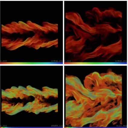
5.10 Optimization results of vortex . . . 100

5.11 Performance of parallel line search . . . 101

5.12 (a) VWS and (b) 2DFS of the vortex data set with a static transfer function only optimized for the first time step . . . 103

5.13 (a) VWS and (b) 2DFS of the vortex data set with a dynamic transfer function optimized for each time step . . . 103

5.14 Time step 30 (a) and time step 80 (b) rendered with a static transfer function only optimized for the first time step . . . 104

5.15 Time step 30 (a) and time step 80 (b) rendered with a dynamic transfer function optimized for each time step . . . 104

5.16 CT-Knee: volume rendered images, transfer functions and VWS graphs 106 5.17 CT-Knee: volume rendered images, transfer functions and VWS graphs 107 6.1 Cloud (a) and precipitation (b) at frame 40 . . . 112

6.2 Volatility of cloud over 5 frames (a), 10 frames (b) and 20 frames (c) at frame 40 . . . 113

6.3 Adjusting saturation and brightness of frame 35 (a), frame 40 (b) and frame 45 (c) . . . 113

6.4 The hurricane at frame 40 . . . 114

6.5 An alternative visualization of the hurricane at frame 35 (a), frame 40 (b) and frame 45 (c) . . . 114

6.7 Smoke density as variable X and gradient magnitude as variable Y at frame 160 . . . 115

A.1 (a) An engine block; (b) and (c) isolated volume rendering images of the red feature and the green feature . . . 124 A.2 The 2D saliency map and feature saliency maps . . . 124 A.3 (a) The residual saliency image; (b) and (c) the Gaussians of the two

feature saliency maps with a kernel size of one eighth of the image width 125 A.4 The residual saliency images of the two features . . . 125 A.5 (a) and (b) The total feature saliency maps of the two features; (c) 2D

Glossary

Entropy

Entropy (or Shannon entropy) is a basic concept in information theory to measure the uncertainty of a random variable.

Feature

A feature in a volume is a subset of voxels in the volume. In this thesis, features are specified by intensity ranges in transfer functions.

Multivariate volume data

Multivariate volume data are volume data that contain multiple variables in each voxel, e.g. a data set containing variables from multiple modalities such as CT, MRI, and PET.

Saliency

Saliency (or visual saliency), for images, is the distinct subjective perceptual quality which makes some regions in an image stand out from their neighbors and immediately grab the user’s attention.

Saliency field

A saliency field for a volume data set represents the saliency (see above) of each voxel in the volume data set. This field itself could be represented in the form of a volume data set.

A saliency model (or saliency map) is a computational model that integrates the normalized information from feature filters for visual properties such as color, intensity and orientation into one global measure of visual saliency.

Saturation

Saturation is a concept in color theory, which refers to the perceived purity or vividness of a specific color.

Time-variant volume data

Time-variant volume is a form of data that typically consists of a series of time-steps (frames) of volume data representing how a system of model changes over time.

Transfer function

Transfer functions are mappings that assign visual properties to volume data. This is a recurrent component of most volume visualization techniques.

Visibility

The visibility of a voxel is the contribution of a voxel to the volume rendered image, which is determined by both the opacity of this voxel and the opacity of those voxels in front of the current voxel in the view direction.

Visibility field

A visibility field for a volume data set represents the visibility of each voxel in the volume data set. This field itself could be represented in the form of a volume data set.

Visibility histogram

Visibility histograms summarize the distribution of visibility of voxels from a given viewpoint. They are feedback mechanisms of volume visualization.

Volume data

Voxel

Chapter 1

Introduction

Volume visualization is an active branch of scientific visualization concerned with ex-tracting meaningful information from volume data (3D discretely sampled data sets) using interactive graphics and imaging. The study of volume visualization involves volume data representation, modeling, manipulation and rendering [8] and it aims, in particular, to facilitate visual exploration of 3D structures allowing users to more deeply understand and analyze volume data sets. First introduced by Levoy [9] in 1988, volume visualization has been widely used in various sciences to create insightful visualizations from both simulated and measured data. However, recent advances in volume data acquisition and scientific simulations have led to dramatic increases in both size and complexity of data sets, which present new and ongoing challenges to be addressed [10].

The rendering of volume data requires every sample value (also called voxel, which is a volume element or volumetric pixel) to be mapped to visual properties (e.g. opacity and color). This mapping is done with a transfer function, which can be a simple ramp, a piecewise linear function or an arbitrary table. The design of an effective transfer function (see Section 2.2 for details) is essential for visualizing volume data.

mod-ifications are made to the transfer function and changes in the resulting visualization are carefully observed in order to inform further modifications to the transfer func-tion [11]. The adjustments users make in transfer funcfunc-tion specificafunc-tion are based on subjective perception of important features in a certain viewpoint.

1.1

Motivation

Objective measures such as voxel information [12], visibility histograms [13] [5], fea-ture visibility [14], and visual saliency models [15] such as saliency maps [16] [17] for 2D images and saliency fields [18] for volumetric data, provide the basis for powerful feedback mechanisms in volume rendering. In current volume rendering systems, ap-propriate transfer functions are often obtained by trial-and-error [19]. It is desirable to take advantage of these objective measures in order to automate the specification of transfer functions for emphasizing features of interest in volume visualization.

The main goal of our research is to investigate the optimization of visualization parameters (in particular transfer functions) with information derived from volume data based on feedback mechanisms from the volume rendering process. We hypothe-size that the importance of voxels (sample values in volume data) are associated with their information content. Therefore, the transfer functions of volume visualization can be optimized based on the information inherent within the data sets and user in-put which indicates the user’s interest. Furthermore, we hypothesize that combining automated optimization techniques with feedback mechanisms such as visibility and visual saliency can provide a more intuitive means for obtaining clear visualization of features of interest in volume data.

1.2

Scope

of transfer functions.

In this research, we focus on the visualization of volume data sets, particularly the scalar field data acquired from medical imaging (e.g. CT and MRI scans) and generated from flow simulations (e.g. computational fluid dynamics).

The features of interest in a volume data set are specified by initial user-defined transfer functions. Therefore, manual segmentation by domain experts or computation-ally expensive automatic segmentation techniques are not in the scope of this thesis. Moreover, this thesis focuses on direct volume rendering techniques. Indirect volume rendering techniques, which require the reconstruction of 3D surfaces, are not in scope of this thesis.

1.3

Contributions

We present a transfer function refinement approach, which exploits the entropy of voxels derived from volume to equalize the opacity transfer function, in order to reduce general occlusion and improve the clarity of layers of structures in the resulting images. Moreover, this approach assists the user in exploring and enhancing features of interest by interactively specifying different priority intensity ranges.

In addition to view-independent information (i.e. entropy of voxels), we propose visibility-weighted saliency for measuring the view-dependent saliency of features of interest for volume visualization. This metric aims to assist users in choosing suitable viewpoints and designing effective transfer functions to visualize the features of interest. (The formal definition of a feature is provided in Section 4.3.1.)

Subsequently, we describe an automated transfer function optimization method based on the visibility-weighted saliency metric. This method takes into account the perceptual importance of voxels and the visibility of features, and automatically adjusts the transfer function to match the target saliency levels specified by the user. In addition, a parallel line search strategy is presented to improve the performance of the optimization algorithm.

1.4

Summary of Chapters

Chapter 2 provides an overview of the background and related work in the field of volume visualization, with particular focus on the design and optimization of transfer functions.

Chapter 3 presents a novel approach for transfer function refinement, which is an optimization of transfer functions based on the distribution (i.e. the histogram) of the volume data. This optimization also allows the user to prioritize specific regions by generating weightings for transfer function components based on user-selected regions. The work described in this chapter has been published as a short paper in Eurographics 2014 [20] and as a full paper in Eurasia 2014 [21].

Chapter 4 describes visibility-weighted saliency as an important measure of visual saliency of features in volume rendered images, in order to assist users in choosing suitable viewpoints and designing effective transfer functions to visualize the features of interest. Visibility-weighted saliency is based on a computational measure of perceptual importance of voxels and the visibility of features in volume rendered images. The visibility-weighted saliency metric has been published as a full paper in Computer Graphics & Visual Computing (CGVC) 2015 [22].

Chapter 5 provides a detailed description of an automated transfer function op-timization approach based on the visibility-weighted saliency metric, which indicates the perceptual importance of voxels and the visibility of features in volume rendered images. The work described in this chapter has been presented as a poster at EG / VGTC Conference on Visualization (EuroVis) 2016 [23].

Chapter 6 outlines a novel visualization approach which modulates focus, empha-sizing important information, by adjusting saturation and brightness of voxels based on an importance measure derived from temporal and multivariate information. The work described in this chapter has been presented as a poster at EG / VGTC Conference on Visualization (EuroVis) 2015 [24].

Related Publications:

1. Shengzhou Luo and John Dingliana, “Visibility-Weighted Saliency for Volume Visualization”, Computer Graphics and Visual Computing (CGVC), London, UK, 2015.

2. Shengzhou Luo and John Dingliana, “Transfer Function Refinement for Exploring Volume Data”, Eurasia Graphics 2014: International Conference on Computer Graphics, Animation and Gaming Technologies, Ankara, Turkey, 2014, p. 17.

3. Shengzhou Luo and John Dingliana, “Information-Guided Transfer Function Re-finement”, Eurographics (Short Papers), Strasbourg, France, 2014, pp. 61–64.

Related Posters:

1. Shengzhou Luo and John Dingliana, “Selective Saturation and Brightness for Vi-sualizing Time-Varying Volume Data”, EG / VGTC Conference on Visualization (EuroVis) 2015 Posters, Cagliari, Italy, 25-29, May 2015.

Chapter 2

Related Work

In this chapter, we present a brief review of the literature related to the concepts that we discuss in this thesis.

2.1

Volume Rendering

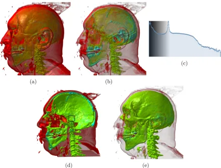
Volume rendering is used to display a two-dimensional (2D) image of three-dimensional (3D) data set. It can be considered as a process of projecting a 3D volumetric data set to a 2D image [25]. The majority of volume data sets are discretely sampled along 3D grids and contain scalar values usually acquired from medical imaging devices such as CT or MRI machines or computed from scientific simulations such as fluid simulation. Volume data sets have the form of 3D arrays and elements in the data sets are called voxels, which are analogues to pixels in 2D images. Figure 2.1 illustrates how voxels (cubic elements) constitute a volume data set. An example of volume rendering is provided in Figure 2.4, which shows a sliced image and a volume rendered image of a head data set.

Traditionally, volume rendering techniques are categorized as either direct volume rendering or indirect volume rendering. Indirect volume rendering is actually surface rendering. It is done by extracting surfaces (polygon meshes) from volume data sets and rendering these surfaces to the screen. A typical method for extracting polygonal meshes from volume data is Marching Cubes [26].

Figure 2.1: Voxels (cubic elements) constituting a volume data set [2].

Figure 2.2: A sliced image of the data set

Figure 2.3: Volume ren-dering of the data set

volume data set as a complete block of data without extracting geometric surfaces from the data [9]. Direct volume rendering consists of a variety of techniques for generating images from 3D scalar fields. Since indirect volume rendering is not in the scope of this thesis, direct volume rendering is henceforth referred to as volume rendering within this thesis.

Volume rendering was initially used in medical imaging, and later became an es-sential technique in many sciences for portraying complex phenomena such as clouds, water flows, and molecular and biological structure [27]. Volume visualization is a synonymous term for volume rendering, sometimes with emphasis on the effective ex-pression of data rather than the realism of rendering.

Motivated by scientific visualization and medical imaging, where volume data is often acquired by devices such as CT and MRI scanners, or numerical simulation of natural phenomena, researchers have developed a wide variety of techniques to improve the performance and enhance the perception of volume visualization [28].

2.1.1

Volume Ray Casting

Volume ray casting is a volume rendering technique that can produce very high quality results. Since the advent of programmable graphics processing units (GPU) and 3D textures, volume ray casting techniques have been able to exploit the power of GPUs to achieve real-time performance. GPU-based volume ray casting has become one of the most popular techniques for visualizing volume data [29]. However, the sizes of volume data are increasing much faster than the sizes of memory available on GPUs [10]. Various scalable volume rendering methods [30] [31] have been proposed to address the challenge of dramatically increasing volume data sizes.

2.1.2

Splatting

Splatting is a volume rendering technique that trades quality for speed by combining volume projection with a sparse data representation [32]. In splatting, only voxels within certain intensity ranges need to be projected and the projection is done with efficient rasterization schemes [33].

2D projection of the kernel is called a splat or footprint. Each voxel’s splat is weighted by its color and opacity specified by the transfer function. Because of the pre-shaded scheme, projecting these fuzzy splats leads to a blurry appearance of object boundaries in the resulting image.

2.1.3

Shear Warp

The shear warp technique [34] consists of three steps. Firstly, a 3D shear is applied to the volume data in directions parallel to the data slices. Secondly, the sheared data is projected to a distorted intermediate image in 2D. Lastly, the intermediate image is warped to produce the final rendered volume image.

Shear warp is relatively fast in software implementation. However, compared to volume ray casting, shear warp has less accurate sampling and potentially worse image quality.

2.1.4

Texture-Based Volume Rendering

Texture-based volume rendering techniques render slices in the volume as texture-mapped polygons with the opacity and color of voxels determined by the transfer function and interpolation and then merge the polygons from back to front in com-positing operations support by the hardware [35]. Because graphics cards are fast at texturing, texture-based volume rendering [36] can efficiently render slices of volume data with the texturing capability of graphics cards.

In 2D texture mapping approaches, slices are aligned with the original volume data. While in 3D texture mapping approaches, slices are aligned with the viewing plane and directly sampled from the 3D volume, which requires graphics hardware support for 3D textures [37].

2.1.5

Illustrative Volume Visualization

Illustrative visualization, as a novel category of visualization, aims to visualize data in a clear and understandable way using techniques from traditional hand-crafted illus-trations. Illustrative visualization has been successfully employed in medical visualiza-tion [40] [41] [42].

Illustration-based styles are believed to be effective in conveying information. Re-searchers in the field of computer graphics and visualization have applied illustration-based styles in order to produce effective and expressive visualization. Stompel et al. [43] introduced feature enhancement techniques, such as strokes-based, temporal domain enhancement, to enhance time-varying data obtained from the field of compu-tational fluid dynamics (CFD).

In scientific visualization, features of interest may often comprise inner structures of the data sets, e.g. visualizing internal organs in anatomical data. In addition, depicting only the features of interest is not sufficient, because the user is often interested in exploring the features within the context of the whole volume data.

(a) Two transfer functions (TF) (b) The result from the TF on the left in (a)

(c) The result from the TF on the right in (a) Figure 2.5: Slight changes in the transfer function causes significant difference in the resulting images [4]

2.2

Transfer Functions

Volume data are 3D entities with information inside them, but the data might not consist of surfaces and edges. Because of the lack of explicit geometric information, it is a major challenge to provide clear visualizations of the structures contained in a volume data set. Volume data may be rendered directly by mapping scalar values to visual properties (e.g. opacity and color), or an intermediate geometric representation may be extracted using techniques like Marching Cubes [26] and then rendered as geometric surfaces. The mapping, which assigns visual properties to volume data, is called a transfer function.

Transfer function specification is an essential part in volume visualization. A simple one-dimensional transfer function is a mapping from scalar values to RGB and alpha values. The resulting visualization largely depends on how well the transfer function captures features of interest [54]. However, it is non-trivial to obtain an effective transfer function. The specification is often achieved by a trial-and-error process, which involves a significant amount of tweaking of color and opacity. Figure 2.5 shows how slight changes in the transfer function lead to significant changes in the resulting images. The adjustment of transfer functions is unintuitive and often difficult.

In practice, major factors that have a great influence on transfer function set-ting are: partial volume effect 1_{, non-uniform distribution of materials and noise [56].}

1_{During the acquisition of data, the finite resolution causes contributions of different materials}

Among these, two challenging problems that need to be tackled could be elaborated as follows: firstly, for volume data sets, e.g. those obtained by MRI and CT, different tissues are represented in similar or even overlapping ranges of scalar values; secondly, interesting interior structures are often partly or completely occluded by surrounding tissue. Consequently, feature detection and understanding volume data become a big challenge.

These problems are handled by transfer functions, which have played a crucial role in volume visualization. Good transfer functions reveal important structures in the data without obscuring them with less important regions. The design of transfer func-tions to generate informative visualizafunc-tions has been a significant challenge addressed by a number of researchers [19]. Various strategies have been proposed for transfer function design [39]. However, features with overlapping intensity intervals are dif-ficult to extract and visualize with 1D transfer functions. When one intensity value or interval is associated with multiple boundaries, a 1D transfer function is unable to render them in isolation [54].

Classical approaches to this problem try to detect boundary information between tissues by introducing derived attributes such as first and second-order derivatives to isolate materials [57] [54]. In this case, the transfer functions are extended to multi-dimensional feature spaces. The introduction of multimulti-dimensional transfer functions alleviates the material separation problem. Instead of classifying a voxel based on a single scalar value, multidimensional transfer functions allow a voxel to be classified based on a combination of values. Multidimensional transfer functions are very effec-tive means to extract materials and their boundaries for both scalar and multivariate data. Multidimensional transfer functions are discussed in more detail in the next subsection.

In addition, various user interfaces were proposed to simplify the design of mul-tidimensional transfer functions [58] [59]. However, the parameter spaces of multidi-mensional transfer functions are more complex (compared to 1D transfer functions) and thus introduce problems such as requirement for large amount of user interaction, missing precision or the interaction being complex and unintuitive [60].

Another strategy is based on the selection of rendered images. This strategy lets the user select one or more favorite images to guide the further search of transfer

functions [61] [62]. More recent approaches introduced visibility [5] [63] or measures derived from information theory [64] [65] [66] [67]. Zhou et al. studied the combination of 2D transfer functions with occlusion and size-based transfer functions [68].

Bruckner and Gr¨oller introduced the concept of style transfer functions [69], which aim to produce more comprehensible images by using transfer functions that map input values to different non-photorealistic rendering styles.

Despite the advances of these methods, transfer function design for volume render-ing is still an open research problem. The creation of transfer functions needs to be simplified and the functionality of transfer functions needs to be extended in order to realize the full potential of volume rendering. For instance, more sophisticated transfer functions are required in medical imaging, in order to address various domain specific visualization problems [70].

Moreover, transfer function specification in general is an unintuitive or even monotonous task for average users, because it usually involves an iterative process of trial and error. For instance, there are skin and fat tissues around the brain, and their intensities lie in the same range as the brain. If we want to visualize the brain by setting the scalar value range of the brain to opaque, the surrounding skin and fat tissue will also become opaque. Then the brain will be occluded by the surrounding soft tissues which make it difficult to explore the brain structure. Common approaches to this problem are to introduce explicit segmentation of structures of interest before the volume rendering process [71]. In fact, the process of applying the transfer function could be interpreted as a segmentation problem.

Multidimensional Transfer Functions

Multidimensional transfer functions [11], which are mappings from intensity and other variables, such as first and second derivatives to color and opacity, have demonstrated their effectiveness in distinguishing boundaries between materials in volume data.

areas [57] [4]. In this case, the transfer functions are extended to multidimensional feature spaces. For higher-dimensional transfer functions, the generation of transfer functions could be memory intensive and costly to compute, and the interaction of transfer functions are more complex and unintuitive as the dimensionality becomes higher.

Therefore, two-dimensional (2D) histograms are often used in multidimensional transfer functions [72]. An example is a 2D histogram with axes representing a subset of the feature space (e.g. scalar value vs gradient magnitude), with each entry in the 2D histogram being the number of voxels for a given feature space pair. Even in the case of two-dimensional transfer functions, a considerable amount of user interaction is required in order to come up with meaningful results [60].

As one of the most common representations of voxel distributions, histograms are used in transfer function design to assign visual properties to voxels [19]. Bajaj et al. [73] introduced the contour spectrum to determine voxels corresponding to important isosurfaces in the volume. To overcome the difficulty of using one-dimensional transfer functions (solely based on scalar values stored in the voxels) to extract inner structures of interest from the volume data, Levoy [9] proposed the use of gradient magnitude to emphasize strong boundaries between different tissues.

The introduction of gradient magnitude as a data metric aims to detect voxels that are of large deviation compared with other voxels by approximating gradient magni-tude at each sample point in the volume, because the exact distribution of data is unknown due to information lost in the discrete sampling process. Kindlmann and Durkin [57] extended Levoy’s work [9] by introducing a higher dimensional transfer function domain based on gradient magnitudes and second derivatives. To emphasize different structures, Kniss et al. [11] presented a technique for interactively manipu-lating 2D histograms of gradient magnitudes and data values. In their work, material boundaries appear as arcs in the 2D histogram and can be selected with interactive widgets [54]. Kniss et al. [74] presented Gaussian transfer functions, which are suitable for the classification of narrow features in multidimensional domains.

Kindlmann et al. [75] proposed curvature-based transfer function to enhance the expressive and informative power of volume rendering. In their approach, volume data is rendered with contours to exhibit constant thickness in image space.

ˇ

selec-tion of boundaries in 2D intensity-gradient transfer funcselec-tions. Subsequently, ˇSereda et al. [77] presented a clustering method based on the LH histograms for semi-automatic transfer function design.

Haidacher et al. [78] described the statistical transfer function space, which is based on statistical properties such as mean and standard deviation of the data values (e.g. intensity and gradient magnitude for 2D transfer functions) in the neighborhood of each voxel. This approach can reduce the influence of noise and enhance visual appearance in volume rendering.

Wang et al. [79] described a clustering approach on 2D density plots for automatic transfer function design. Their approach allows the user to interactively explore the pre-computed clusters in the feature space and merge or remove uninterested features to improve visualization quality. Ip et al. [80] described a multilevel segmentation technique that mimics user exploration behaviors by recursively segmenting intensity-gradient histograms.

There are other multidimensional transfer function approaches, such as spatialized gradient-based transfer functions [81], distance-based transfer functions [82], size-based transfer function [83], texture-based transfer functions [84] [85].

In addition, parallel coordinates and dimensionality reduction algorithms (e.g. prin-cipal component analysis) have been employed to support the design of transfer func-tions in multidimensional parameter spaces [86] [87] [88].

2.3

Automated Transfer Function Generation

Researches have proposed various approaches to automate the design of transfer func-tions and provide acceptable suggesfunc-tions which can be further edited by users. How-ever, the usefulness of a transfer function mostly depends on the underlying question the user wants to answer. Moreover, users’ tasks vary drastically from one domain to another. Therefore, most techniques work semi-automatically and very few techniques consider domain knowledge in the design process [89].

rendered images as feedback, in order to achieve desired results. Marks et al. [61] pre-sented Design Gallery, which lets the user select one or more favorite images to guide the further search of transfer functions. Rezk-Salama et al. [91] presented high-level semantics to abstract parametric models of transfer functions in order to automatically assign transfer function templates.

Wu and Qu [62] developed a method that uses editing operations and stochastic search of the transfer function parameters to maximize the similarity between volume-rendered images given by the user. Maciejewski et al. [72] described a method to structure attribute space in order to guide users to regions of interest within the transfer function histogram. Chan et al. [92] developed a system to optimize transparency automatically in volume rendering based on Metelli’s episcotister model to improve the perceptual quality of transparent structures. Correa and Ma [5] proposed the visibility histogram to guide the transfer function design.

Zhou and Takatsuka [93] presented an automated approach for generating transfer functions, which can depict inclusion relationships between structures in the volume, and maximize opacity and color differences among the structures. This approach uses a residue flow model based on Darcy’s Law to differentiate the distribution of opacity be-tween branches of a contour tree. Selver and G¨uzeli¸s [94] introduced a semi-automatic method for transfer function initialization and optimization using volume histogram stacks and radial basis function networks.

Inspired by how physicians interact with volume data to extract clinically relevant information, L¨ath´en et al. [95] proposed an optimization method for shifting transfer function presets, in order to better visualize contrast enhanced blood vessels.

Maciejewski et al. proposed a non-parametric method to generate transfer functions [72]. In their later work [96], instead of using the attributes, metrics representing relationships and correlations in the underlying data were used in the method.

2.4

Visibility Histograms and Visibility-Driven

Trans-fer Functions

In traditional transfer function design, the visibility of structures revealed in vol-ume rendering is a consequence of adjusting transfer function parameters, rather than a design parameter [98]. Correa and Ma [5] introduced visibility histograms to guide transfer function design for both manual and automatic adjustment. Visibility his-tograms (Figure 2.6), which summarize the distribution of visibility of voxels from a given viewpoint, are powerful feedback mechanisms of volume visualization [13]. Vis-ibility histograms encode the information required to measure the efficacy of transfer functions and are advantageous in guiding and automating the manipulation of transfer functions.

Wang et al. [6] extended the previous work on visibility histograms and proposed a feature visibility metric, in order to measure the influence of each feature to the volume rendered image. As shown in Figure 2.7, their approach allows the user to directly specify the desired visibility for the features of interest, and subsequently the opacity transfer function is optimized using an active set algorithm [99].

Ruiz et al. [66] proposed an information-theoretic framework which obtains opacity transfer functions by minimizing the Kullback-Leibler divergence between the observed visibility distribution and a target distribution provided by the user. Later, Bramon et al. [67] extended this approach to visualize multimodal volume data.

Cai et al. [100] described a method to derive opacity transfer functions by minimiz-ing the Jensen-Shannon divergence between the observed visibility distribution and a user-defined target distribution. The target distribution can be defined using Gaussian function weighting.

In addition, various methods were proposed regarding the use of visibility for en-hancing different aspects of volume visualization. Marchesin et al. [101] introduced a volume rendering technique that manipulates the voxel opacity values in a view-dependent way, in order to enhance visibility of internal structures in the volume data set. Bronstad et al. [102] described local opacity transfer functions with feature de-tection along the ray profile implemented on the GPU. In their approach, visibility histograms are employed to access the performance of the feature detection algorithm.

(a) A user-defined opacity transfer function and the initial visibility histogram

(b) Here the visibility histogram has been modified to match the user-defined opacity transfer function.

together with region of interest segmentation was effective in visualizing PET-CT vol-ume data sets.

Instead of computing the visibility of all voxels, Zheng et al. [105] employed local visibility histograms to ensure both the features of interest and contextual information are visible in multimodal volume visualization. Schlegel and Pajarola [106] proposed a visibility-difference entropy metric. They presented an automated approach using this metric for generating a set of transfer function candidates with high ratings and are strongly distinct in what they reveal.

Qin et al. [107] presented the voxel visibility model as a quality metric for transfer function design. The voxel visibility model is a mapping function from data attributes of voxels to their visibility attributes. Instead of specifying transfer functions, this approach allows users to directly adjust the visibility of each voxel, and then the corresponding opacity transfer functions can be obtained by minimizing the distance between the desired voxel visibility distriubtion and the actual voxel visibility distri-bution.

2.5

Multivariate Volume Visualization

Analyzing multivariate data is an importance and challenging topic in many scientific disciplines. For instance, applications in medicine, engineering and meteorology often require analyzing multivariate data. However, multivariate volume data sets are usually mapped to a scalar dimension and visualized separately with standard volume rendering techniques. Because of the disparity in data resolutions and higher computation and storage requirements, simultaneous visualization of multiple variables in volume data is more challenging than standard volume visualization [108].

Stompel et al. [43] demonstrated feature enhancements using non-photorealistic ren-dering and hardware-accelerated techniques to generate perceptually effective visual-ization of multidimensional and multivariate volume data sets. Kniss and Hansen [109] applied volume rendering with multidimensional transfer function to visualize multi-variate weather simulations. In their approach, they combined the temperature and humidity as a multivariate field in order to assist the meteorologists in identifying the frontal zones.

classifica-tion of time-varying data in order to find transfer funcclassifica-tions that classify all the time steps of the data set. Woodring and Shen [111] presented a method for the compari-son of different data fields through the expression of a volume shader that composes data fields together with set operations. Wang et al. [112] introduced an importance measure based on conditional entropy and categorize temporal behaviors by clustering the importance curves over time.

Lee and Shen [113] introduced dynamic time warping (DTW) to measure the shape similarity between two time series with an optimal warping of time in order to ac-count for the phase shift of the feature in time. Subsequently, they extended DTW to SUBDTW [114], in order to estimate when a trend appears and vanishes in a given time series. They modeled the temporal relationships as a state machine based on the beginning and ending times of the trends.

Khlebnikov et al. [115] described a novel method that allows simultaneous rendering of multivariate data by redistributing the opacity within a voxel. This method uses procedural texture synthesis [116] for opacity redistribution pattern and is similar in spirit to color weaving.

Data analysis techniques for high dimensional spaces, such as parallel coordinates [117] [118] and principal component analysis [119], were also investigated for exploring multivariate time-varying data sets.

2.6

Time-Varying Volume Visualization

Although researchers have developed a great number of visualization techniques for static volume data [19], how to effectively explore and understand time-varying volume data remains a challenging problem. Finding good transfer functions for time-varying volume data is more difficult than for static volume data, as data value ranges and distributions change over time.

2.6.1

Transfer Functions for Time-Varying Volume

Visualiza-tion

set in order to obtain coherent visualization. More than one color or opacity map can be misleading or physically meaningless, because the transition from one transfer function to another may cause sudden changes in the resulting images. However, the practice of using a single transfer function is not always applicable to general time-varying data sets. In some cases, the intensity distributions change significantly over time, thus applying a single transfer function to all frames becomes ineffective.

Volume data sets are inherently 3D representations. Automated analysis meth-ods, such as temporal trends or statistical aggregates e.g. mean values and standard deviations, are often applied in order to abstract dynamic characteristics of the data sets [120]. Jankun-Kelly and Ma [121] examined how to combine transfer functions for different time-steps to generate a coherent transfer function. Woodring et al. [122] considered time-varying volume data as four-dimensional data field and provided a user interface to specify hyperplanes in 4D. Woodring and Shen [123] introduced an alternative approach to render multiple time-steps in a sequence with different colors into a single image. This approach provides the context of surrounding time steps but coherence of color among time-steps is hard to maintain.

Tikhonova et al. [124] presented an exploratory approach based on a compact rep-resentation of each time step of the data set in the form of ray attenuation functions. Ray attenuation functions are subsequently used for transfer function generation. Ak-iba et al. [110] introduced the time histogram which allows simultaneous classification and specification of temporal transfer functions for the entire time series.

A time-varying volume data set can be considered as a 3D array where each voxel contains a time-activity curve (TAC). Fang et al. [125] described an approach for classi-fying time-varying volume data based on the temporal behavior of voxels and three dif-ferent similarity measures that can be used in their approach. Woodring and Shen [126] presented a method that filters time-varying volume data into several time scales using a wavelet transform and classifies the voxels by clustering the entire time series by time scale. Lee and Shen [113] proposed a method for classifying time-varying features using time activity curves with the dynamic time warping distance metric.

Ward and Guo [128] presented a method for visualizing time-series data that re-veals a wide variety of features in the data, by mapping short sub-sequences of the time-varying volume data into a high-dimensional shape space, and then performing a dimension reduction process to allow projection into screen space.

Gu and Wang [129] proposed an approach to organize a time-varying data set into a hierarchical graph, which captures the transition relationships in the data set. This approach assists the user in comprehending the correspondence between volume regions over time and allows interaction of the graph through brushing and liking.

In order to create coherent and feature-prominent animations of time-varying vol-ume data, Peng et al. [130] described an optimal color mapping strategy, which uses a two-phase optimization method with bilateral filtering and energy minimization.

2.6.2

Visualizing Time-Varying Volume Data with

Non-Photorealistic Rendering

In contrast to traditional computer graphics, which has focused largely on creating photorealistic images of synthetic objects, non-photorealistic rendering is an area of computer graphics that focuses on creating abstract images with a wide variety of ex-pressive styles [131]. In certain situations, non-photorealistic renderings are considered more effective and expressive than an equivalent photograph [132].

An essential problem in time-varying volume visualization is to visualize temporal variation and analysis of features. Traditionally, time-varying data has been visualized as snapshots of individual time steps or as an animation of snapshots of a sequence of time steps. These techniques are effective in making time-varying data understandable, however, they struggle when the complexity of data sets increased dramatically in recent years [133].

boundary enhancement, oriented feature enhancement (silhouettes, fading, and sketch lines). The techniques in the second category focus on illustrating dynamic aspects such as movement of features. A number of techniques have been proposed for this purpose. For example, there are speed lines, flow ribbons and strobe silhouettes, which are inspired by traditional animation [135] [136] [137]; and there are extended silhou-ette and boundary enhancement domains, which are inspired by the techniques used by illustrators and other artists [40]. Nevertheless, illustrations of temporal features of time-varying data requires more attention from researchers in the visualization com-munity. The usefulness of illustrative approaches in time-varying volume visualization has not been studied as thoroughly as in other areas.

2.6.3

Vector Field Visualization

The visualization of vector fields plays a crucial role in visual interpretation and under-standing of the underlying flow features and patterns [138] [139]. Since flow patterns also exist in time-varying volume data, certain techniques for visualizing vector fields could be incorporated into time-varying volume visualization, in order to depict the dynamic aspects of time-varying data.

Line drawings are effective ways to depict complex information with simple means [140]. Among vector field visualization techniques, streamline visualization is a simple but common way to convey the structure of 3D vector fields [141]. Streamlines have proven to be expressive in vector field visualization if they are combined with appro-priate seeding strategies [142]. Texture patterns generated by line integral convolution are used in 2D vector field visualization. Rezk-Salama et al. [143] introduced volume rendering as a means to efficiently render 3D line integral convolution for visualizing 3D vector fields.

2.6.4

Feature Tracking

In practice, feature extraction and tracking are often employed in the exploration and analysis of time-varying volume visualization in order to better understand the dy-namic nature of the underlying phenomena [146] [126] [113]. Feature extraction meth-ods are often based on an analytic description of the feature of interest. Consequently, feature extraction and tracking could become manual-driven and trial-and-error pro-cesses when properties cannot be easily defined or unknown [147].

Tzeng and Ma [148] proposed an intelligent feature extraction and tracking al-gorithm, which applies machine learning to extract and track time-varying fluid flow features in volume data. They investigated the use of both neural networks and support vector machines in their approach and obtained promising results.

Based on the observation that regions in time-varying volume data present specific pattern and textural features, Caben et al. [149] introduced a texture-based feature tracking technique which analyzes local textural properties and finds correspondent features in the time series. Caban and Rheingans [84] extended this technique for transfer function design, in which the voxels’ resulting opacity and color are based on local textural properties instead of intensity values.

Gu and Wang [150] described the TransGraph, which is a graph-based representa-tion for visualizing hierarchical state transirepresenta-tion relarepresenta-tionships. This approach provides an occlusion-free overview map and allows controllable interaction to help users to track data transition over space and time.

Hsieh et al. [151] introduced a particle swarm method for transfer function design. This method maps the frequency of particle occurrences to color and opacity values, and extracts features after the particles finish searching for features in the volume data.

2.7

Information Theory in Visualization

Information theory [154] was originally introduced to study the fundamental limit of reliable transmission of messages through a noisy communication channel. In infor-mation theory, inforinfor-mation is considered as a set of possible messages, where the goal is to send the messages through a noisy communication channel and then to have the messages reconstructed with low probability of error.

Traditional applications of information theory, such as data compression and data communication, focus on the efficient throughput of a communication channel, while visualization focuses on the effectiveness in aiding the perceptual and cognitive process for data understanding and knowledge discovery [155].

In recent years, there is an emerging direction towards using the principles of infor-mation theory to solve challenging problems in scientific visualization [14]. These prob-lems include view selection [12] [156] [157], streamline seeding and selection [158] [159], transfer function for multimodal data [160], representative isosurface selection [161], time-varying and multivariate data analysis [112] and information channel between objects and viewpoints [162].

Chen and J¨anicke [163] presented an information-theoretic framework for visual-ization. Examining the theoretical aspect of information and its relation to data com-munication, they interpreted different stages of the visualization pipeline using the taxonomy of information.

Haidacher et al. [64] proposed an approach for transfer function specification for multimodal data visualization. They considered the joint occurrence of multiple fea-tures from one or multiple variables in order to separate statistical feafea-tures that only occur in a single variable from those that are present in both.

Wang et al. [112] introduced an approach to characterize the dynamic temporal behaviors of spatial blocks using importance curves, which are based on conditional entropy. Clustering is performed on the importance curves of all the spatial blocks to classify the underlying volume data set.

Ruiz et al. [66] presented an approach to generate transfer functions from a target distribution provided by the user. Their approach is based on a communication channel between a set of viewpoints and a set of bins of a volume data set, and supports both 1D and 2D transfer functions including the gradient information.

Bramon et al. [67] proposed an automatic method to visualize multimodal data by combining several information-theoretic strategies to define colors and opacity values of the multimodal transfer function. They set an information channel between two registered input data sets to define the fused color and minimize the informational divergence between the visibility distribution captured by a set of viewpoints and a target distribution proposed by the user to obtain the opacity.

2.8

Computational Saliency in Visualization

Predicting salient regions in images [164] can be exploited as useful feedback for im-proving visualizations. Inspired by mechanisms of the human visual system, various computational models of visual saliency have been proposed to predict gaze allocation in an image [16] [165] [17] [166] [167] [168].

J¨anicke and Chen [169] described a quality metric for analyzing the saliency of visualization images and demonstrated its usefulness with examples from information visualization, volume visualization and flow visualization. Corcoran et al. [46] com-pared the effectiveness of various stylized volume visualization techniques on the basis of shape perception.

Kim et al. [170] extended their previous work on detecting salient regions in images [171] to detect salient regions in both images and videos. Both approaches use the self-ordinal resemblance measure to compute the spatial saliency. Then the spatiotemporal saliency map is generated by combining the spatial saliency with the temporal saliency, which is the sum of absolute differences of temporal gradients of the center and the surrounding regions.

approach was better at eliciting viewer attention than the traditional Gaussian regional enhancement approaches.

Shen et al. [173] proposed the use of saliency to assist volume exploration. They described a method for inferring interaction position in volume visualization, in order to help users pick focused features conveniently. Shen et al. [174] described spatiotemporal volume saliency, which extended the saliency field [18] to time-varying volume data.

2.9

Perceptual Evaluation

Traditional, visualization research has an emphasis on solving problems with modeling and optimization using engineering and mathematics tools. A recent focus in visual-ization has become measuring the effectiveness of a proposed method with adequate user studies [175]. Due to the complex nature of the data being studied, simply dis-playing all available information does not adequately meet the demands of domain scientists [176]. User studies can be used to evaluate the strengths and weaknesses of visualization methods [177]. The evaluation of visualization methods that focus on hu-man factors often employ user studies or expert evaluations to determine their effects on interpretation and usability.

There are a number of different evaluation strategies, such as measuring user per-formance, accuracy and experience [178]. Laidlaw et al. [179] compared six methods for visualizing 2D vector fields and measured user performance on three flow-related tasks for each of the six methods. They used the evaluation results to identify what makes a 2D vector fields visualization effective. Joshi and Rheingans [136] evaluated the effective of their illustrative techniques by measuring user accuracy, time required to perform a task and user confidence.

Lu [180] described a method for automatically selecting rendering parameters to simplify user interaction and improve usability. Subsequently, a user study was con-ducted to evaluate the effectiveness of this method. Two data sets were rendered in three styles with three predefined portions of the data sets were highlighted respec-tively. The users’ eye gaze patterns were analyzed to determine if they were able to accurately identify the highlighted areas in the images.

determine which one of two indicated vessels was closer to them, and were asked to respond as accurately and quickly as possible. Both the percentage of correct answers and response times were analyzed.

Also for depth perception, D´ıaz et al. [182] conducted a user study to investigate the impact of well-known volumetric shading models [183] in stereoscopic desktop-based environments. In the results, the average time spent and average correctness of answers were analyzed.

2.10

Summary

We have presented a review of literature in the field of volume visualization. Specific areas which were reviewed in detail include transfer functions, automated transfer func-tion generafunc-tion, visibility histograms, informafunc-tion theory and computafunc-tional saliency. Transfer functions are relevant to all of the following chapters as transfer function optimization is a central theme of this thesis. Information theory is relevant to Chap-ter 3. Visibility and computational saliency are relevant to ChapChap-ter 4 and ChapChap-ter 5. Transfer functions for time-varying volume visualization relates to Chapter 6

Chapter 3

Information-Guided Transfer

Function Refinement for Exploring

Volume Data

In this chapter, we describe a global optimization and two user-driven refinement meth-ods for modulating transfer functions in order to assist the exploration of volume data. This optimization is dependent on the distribution of scalar values of the volume data set and is designed to reduce general occlusion and improve the clarity of layers of structures in the resulting images. The user can explore a volume by interactively specifying different priority intensity ranges and observe which layers of structures are revealed. In addition, we show how the technique can be applied to time-varying vol-ume data sets by adaptively refining the transfer function based on the histogram of each time-step. Experimental results on various data sets are presented to demonstrate the effectiveness of our method.

3.1

Introduction

set and thus affect which structures will be visible to the user. However, obtaining an effective transfer function is a non-trivial task, which often entails time-consuming tweaking until a desired aesthetic quality is achieved in the resulting rendering. Al-though a number of automatic or semi-automatic approaches have been developed, transfer function design remains a challenging problem [19] [60].

For end users, such as physicians, who may not have much experience in volume rendering and transfer function design, a user-friendly approach that allows them to intuitively explore volume data sets is very desirable. As fully automatic approaches cannot currently guarantee satisfactory results in every case, exploratory approaches with simple and efficient interaction are highly desirable.

We propose a novel approach to refine the transfer function based on the distribution of the scalar values of the volume data set. Firstly, we propose an automatic step to refine the transfer function that improves the rendering of volume data by reducing overall occlusions with no previous assumptions of the data set. Furthermore, we propose two interactive methods that extend on the optimization technique in order to enhance specific intensity ranges within the data as identified by the user. The process is fast and intuitive and allows the user to provide customized views of the data to aid in visual exploration of the volume data set.

3.2

Related Work

A number of approaches have been proposed to automate the design of transfer func-tions, and these are discussed in detail in Section 2.2. Here, we briefly discuss the most closely related previous works to the contribution of this chapter.

air fat soft tissue bone (cancellous/dense) -1000 -100 to -50 +100 to +300 +700 to +3000

Table 3.1: Hounsfield units of some typical substances [1]

as a main parameter for the transfer function specification. Their method obtains the opacity transfer function by minimizing the informational divergence between the visibility distribution captured by a set of viewpoints and a target distribution defined by the user. Later, Bramon et al. [67] extended this approach to deal with multimodal information.

3.3

Background

3.3.1

Transfer Function Specification

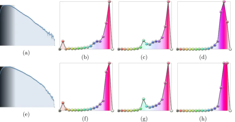
In the specification of a 1D (intensity-based) transfer function, the user essentially assigns a color and/or opacity to a certain point in the histogram of scalar values in the data set. In practice, the user would be presented with an interface that allows them to set up several control points which corresponds to a certain kind of material or structure. The user then defines a mapping from each control point to some visual property (e.g. color) resulting in voxels of the corresponding intensity to be rendered in that color. Figure 3.1 displays four typical shapes used in transfer function design. If a volume data set contains complex structures, tent-like shapes are desirable in revealing isosurfaces of structures and seeing through inner structures. Otherwise, the ramp shape and other shapes can also reveal structures effectively.

In order to design transfer functions effectively, it is commonly required that users have prior knowledge about which intensity ranges are relevant or which regions should be emphasized in the data. This is especially the case in medical visualization. For instance, in computed tomography (CT) data the intensity ranges are determined by the Hounsfield scale (Table 3.1). The user may expect the constituent’s intensity of CT data to follow the Hounsfield scale and thus set up control points accordingly.

Figure 3.1: Typical transfer function shapes [7]