R E S E A R C H
Open Access
A stabilized coupled method and its optimal
error estimates for elliptic interface problems
Jiaping Yu
1,2, Feng Shi
3*and Jianping Zhao
4,5*Correspondence: [email protected]
3College of Science, Harbin Institute
of Technology, Shenzhen, China Full list of author information is available at the end of the article
Abstract
In this paper, we present a stabilized coupled algorithm for solving elliptic interface problems, mainly by introducing the jump of the solutions along the interface. A framework of theoretical proofs is provided to show the optimal error estimates of this stabilized method. Several numerical experiments are carried out to demonstrate the computational stability and effectiveness of the method.
Keywords: The interface problem; Stabilized method; Couple method; Optimal error estimates
1 Introduction
The interface problem has always been a difficult issue in multi-physics and multi-phase applications in science and engineering and has becoming focused recently. In real physi-cal world, many phenomena need to be described using non-smooth or even discontinu-ous functions/methods. A lot of methods have been put forward to improve the standard numerical methods which may not be applied directly. Focusing on the approximation of non-smooth solutions related to the present work, there are mainly two fundamentally different approaches.
One approach of improvement is to enrich the approximation space or discrete form, for instance, the immersed boundary method (IBM) [1], the immersed interface method (IIM) [2–5] and some modified methods for them in the finite difference method (FDM). This type of methods usually incorporates the interface conditions into the finite difference scheme near the interface to achieve second- or higher-order accuracy based on a Taylor expansion in a local coordinate system. Concentrated on the development of the high-accuracy or augmented method [6], these methods can treat the irregular domain problem on a rectangular domain so that fast solvers for Poisson/Helmholtz equations can be used. Several methods of finite element versions, such as the immersed interface finite element method (IIFEM) [7,8], the weak Galerkin finite element method [9], the extended finite element method (XFEM) [10,11], the generalized finite element method (GFEM) [12], and non-traditional finite element methods [13,14] have also been developed. These methods usually modify the basis function or add virtual nodes near the interface.
Another approach of improvement is to refine the discretization near the critical re-gions, so the procedure of re-meshing is usually required in this case. For instance, by placing more grid-points along the interface and around the intersection. Bernardi and
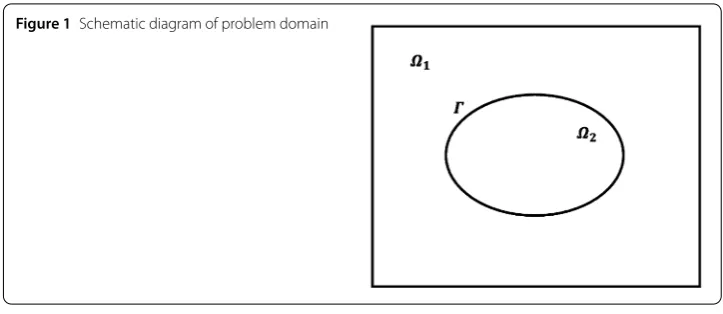
Figure 1Schematic diagram of problem domain
Verfurth proposed weighted-residual error estimators to deal with interfaces [15] and Cai and Zhang proposed recovery-based error estimators [16,17]. Note that, in the previous method, the meshes were generated along the interface.
For many numerical methods, researchers often use stabilization to reduce the error [18], which inspires us to solve the interface problem in such way. By combining the two-level method and the partition of unity, the authors and their collaborators proposed two local and parallel algorithms for the Stokes problem [19], elliptic equations [20], the Stokes–Darcy model [21] and the fluid–fluid model [22,23]. In this paper, we consider the elliptic interface problem as a mixed elliptic–elliptic model. We will introduce the jump of the solution along the interface as our stabilization term of the stabilized method and then obtain the optimal error estimates for the method.
The rest of the article is organized as follows. In Sect.2, some preliminary notations and inequalities are introduced. As the main parts of this paper, in Sect.3and4, the stabilized coupled algorithm and its analysis are discussed. Then numerical tests are presented in Sect.5. Finally, some conclusions are given in Sect.6.
2 Preliminaries
In this section, we will introduce some basic notations and inequalities. LetΩ⊂Rd(d= 2, 3) be a bounded domain with Lipschitz boundary andΩ=Ω1∪Γ∪Ω2. HereΩ1andΩ2 are two disjoint subdomains which are either convex or of classC1,1, and coupled by a fixed interfaceΓ ⊆∂Ω(see Fig.1for example). Both boundaries∂Ω1,∂Ω2and interfaceΓ are assumed to be polygonal (d= 2) or polyhedral (d= 3) for the sake of avoiding analyzing the effect caused by triangulation of domain into finite elements [24]. For any domainD, we denote the norm for the Sobolev spaceHk(D) by ·
k,D withk> 0 (see for instance
[25]). Whenk= 0, we denoteW0,m(D) connected with the norm ·
Lm(D) byLm(D). In particular,W0,2(D) with the norm ·
0,Dis denoted byL2(D). The definitions of the space H
1 2
00(Γ) and its dual spaceH –12
00 (Γ) will also be used and are referred to [26]. We then define two spaces by
Xi=vi∈H1(Ωi);vi|∂Ωi\Γ = 0
, i= 1, 2,
and their tensor space by
Fori= 1, 2, letπhibe a regular partition of each subdomainΩi, which consists ofKthat
are tetrahedral elements ford= 3 and triangles ford= 2. We denote the diameter of the elementK∈πh=πh1∪πh2byhK and mesh scaleh=maxK∈πhhK. Accordingly, we define the following finite element spaces onπhi:
Xi,h=Xi∩
vi,h∈H1(Ωi);vi,h|K∈Pk(K),K∈πhi
⊂Xi, i= 1, 2,
wherePk(K) is the space of polynomials of orderkonKwithk≥1, and tensor space
Xh:=X1,h×X2,h⊂X.
Some useful inequalities are listed in the end of this section. We refer to [26,27] for such inequalities.
A1: (Trace inequality) For anyvi∈Xi,
viΓ ≤ ˜Ctrvi
1 2
0vi
1 2
1. (1)
A2: (Interpolation inequalities) For anyui∈Xi∩Hk+1(Ω
i)withk≥1, there exists Ihui∈Xi,hsuch that
ui–Ihui0,Ωi+hui–Ihui1,Ωi≤CIh k+1u
ik+1,Ωi. (2)
3 The elliptic interface problem
The model of the elliptic interface problem considered in this paper is as follows:
–∇ ·(νi∇ui) =fi, inΩi,i= 1, 2, (3)
ui= 0, on∂Ωi\Γ, (4)
u1–u2= 0, onΓ, (5)
n1·ν1∇u1+n2·ν2∇u2=g, onΓ. (6)
Here fori= 1, 2,niis the unit outward normal toΓ of domainΩi,f is the given source
term, anduiis the restriction ofuinΩi.
The variational formulation of the problem (3)–(6) is: for any givenh, findui∈Xi satis-fying
ai(ui,vi) + δ
h
Γ
(u1–u2)(v1–v2)ds
–1 2
Γ
(ν1∇u1·n1–ν2∇u2·n2)(v1–v2)ds
= (fi,vi) +1 2
Γ
gv1ds+ 1 2
Γ
gv2ds, ∀vi∈Xi,i= 1, 2, (7)
where
Since in the present situationu1–u2= 0 onΓ, we actually add a zero term δh
Γ(u1– u2)(v1–v2)dsin the variational formulation to (3)–(6) comparing with the standard weak formulation. However, this modification will be very useful and important as shown in our later analysis in the next section and also numerical simulations.
By introducing some important notations for u = (u1,u2), v = (v1,v2)∈X
the above variational formulation (7) can be equivalently rewritten as: Find u∈X satisfy-ing
We also need the inverse and trace inequality as follows [26,27]:
vi,hΓ ≤ ˜Cinvh–1/2vi,h0, ∀vi,h∈Xi,h. (9)
4 The coupled algorithm for the interface model and error estimates
In this section, we will present our algorithm for solving the coupled problem (3), which is referred as the coupled scheme.
Algorithm 1(The coupled scheme) Findui,h∈Xi,h,i= 1, 2, such that
Remark1 In the present work, to keep the briefness of introducing our coupled method and proving its optimal error estimates, we only consider both homogeneous non-interface boundary condition (4) and homogeneous interface jump condition (5). The extension to the general conditions ui=φi, on∂Ωi\Γ,u1–u2=ψon∂Γ as studied in [9] is trivial. Actually, we only need modify two places in the numerical scheme (10): (i) addinghδΓψ(v1,h–v2,h)dsin the right side of (10); (ii) replacing solution spacesXi,hby
We can also equivalently rewrite this scheme as: Find uh∈Xhsatisfying
In the remaining part of this section, we will focus on deriving the optimal error esti-mates for the coupled Algorithm1. Actually, Theorem1and Theorem2will provide the error estimates of the numerical solutions inH1norm andL2norm, respectively.
Theorem 1 Letube the solution of the variational formulation(8)anduh be the finite element solution deduced by Algorithm1.Under the hypothesis thatu∈X∩Hk+1(Ω),the
following estimate holds:
u– uh1,Ω≤Chk. (12)
Proof For convenience, we separate the errors into two parts,
ui–ui,h= (ui–Ihui) + (Ihui–ui,h) :=φi+θih, i= 1, 2.
Then by denotingΦ= (φ1,φ2),Θh= (θ1h,θ2h), we obviously have
u– uh=Φ+Θh.
Subtracting (11) from (8) gives the error equations as
a(u – uh, vh) +
Using the inverse inequality (9), the Hölder inequality and denoting two positive con-stants
we can derive the following estimates for (14):
δ
Then combining (14) with (15)–(18), and applying the trace inequality A1, we can obtain
1
here C0 is defined as a constant associated with the equivalence of two norms onΩ, namely,∇(·)0≤C0 · 1.
From (19), we can see that if selectingδ≥4C˜2
invνmax, by interpolation inequality A2
νmin
Due to the triangle inequality and the interpolation inequality A2, we finally arrive at
∇(u – uh)0≤∇Θh0+∇Φ0≤Chk, (22)
cannot be too large to ensure a good approximation result. Compared with the term before
δinC, we can select
Remark 2 For the stabilization parameter δ selected above, we always have C≤[1 + (5C0ννmaxmin)
1/2]C
Iuk+1,Ω, which is independent of the mesh sizeh.
In the end, we present the error estimate inL2(Ωi) for the coupled scheme.
Theorem 2 Letube the solution of the variational formulation(8)anduh be the finite
element solution deduced by Algorithm1.Assuming thatu∈X∩Hk+1(Ω),we have the following estimate:
u– uh0≤Chk+1. (25)
Proof Firstly we construct a dual problem of (3) as follows:
–∇ ·(νi∇zi) =ui–ui,h, inΩi,i= 1, 2, (26)
zi= 0, on∂Ωi\Γ, (27)
z1–z2= 0, onΓ, (28)
n1·ν1∇z1+n2·ν2∇z2=r, onΓ. (29)
Choosingr= 0, we have
u– uh20=a(z, u – uh) + δ h
Γ
[z][u – uh]ds
–1 2
Γ
[ν∇z·n][u – uh]ds. (30)
Thanks to (13), we know that
u– uh20=a(z –Ihz, u – uh) + δ h
Γ
[z –Ihz][u – uh]ds
–1
2 ν∇(u – uh)·n
, [Ihz]Γ –1 2
Γ
[ν∇z·n][u – uh]ds. (31)
Noting that [Ihz] = 0, [ν∇z·n] = 0 onΓ, by the Hölder inequality, the trace inequality A1 and the interpolation inequalities A2, we can obtain that
u– uh20=a(z –Ihz, u – uh) + δ h
Γ
[z –Ihz][u – uh]ds
≤C∇(z –Ihz)0∇(u – uh)0+ Cδ
h z–IhzL2(Γ)u– uhL2(Γ)
≤Chz2∇(u – uh)0+Cδh1/2z2u– uh1/20 ∇(u – uh)1/20 . (32)
Since the domain and the interface are both convex, we can derive from (26) that, while
r= 0,
Then we arrive at
u– uh20
≤Chu– uh0∇(u – uh)0+Cδh1/2u– uh03/2∇(u – uh)1/20
≤Ch2∇(u – uh)
2 0+
1
2u– uh 2
0, (33)
which immediately yields
u– uh0≤Chk+1.
The proof is completed.
5 Numerical tests
In this section, several numerical examples are carried out to illustrate our theoretical results. We select the stabilization parameterδ= 1.0 in the first three testing examples, and
δ= 0.1 in the last case. The code is implemented and executed using the software package FreeFEM++ [28]. The linear solver UMFPACK is used for solving linear equations of the resulting system discretized by the finite element method for (10).
Example1 Firstly we consider a stationary heat conduction problem in a single solving domainΩ= [0, 1]×[0, 2] with analytic solution as follows:
u=2 –πsin(πx)1 –y–cos(πy).
By introducing a straight internal boundaryΓ = (0, 1)× {1}, we divide the domainΩinto two subdomainsΩ1= [0, 1]×[0, 1] andΩ2= [0, 1]×[1, 2]. In this exampleg= 0 in (3),
ν1=ν2, and the right hand sidesfiand other boundary conditions are derived from the
exact solution. To this end, we can say that the present algorithm can be regarded as a special domain decomposition method for this problem.
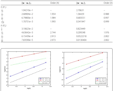
A sequence of uniform triangular meshes are generated by aligning with the interface
Γ. Based on these meshes, theH1andL2 errors for numerical solutions by the present method are reported in Table1withP1(k= 1, linear) andP2(k= 2, quadratic) elements. From this table and the plotted convergence results in Fig.2, the numerical orders ofk
andk+ 1 respectively in the sense ofH1andL2norms are observed clearly.
Noting that in general,u1–u2=ψ is usually not zero. However, in the non-zero case, we only need to add another additional term in the right hand side related toψ, which will not obviously affect our analysis sinceψis some prescribed function. To this end, we follow [29] in the next three examples to carry out our testings to verify theoretical results. For simplicity, we only consider theP1element hereafter.
Example2 Now we consider a circular interface problem. The domainΩ1consists of a circle with its center at the origin and a radius of 0.5. LetΩ= [–1, 1]×[–1, 1] andΩ2=Ω\
Ω1. The coefficientsνifor different domainsΩiare chosen asν1= 10,ν2= 1, respectively. The analytical solution is chosen as
Table 1 Convergence order with respect tohof the stabilized method for Example1withP1andP2 elements
u–uh0 Order (h) u–uh1 Order (h)
h(P1) 1
16 1.04210e–1 – 2.70631 –
1
32 2.68904e–2 1.954 1.36429 0.988
1
64 6.79800e–3 1.984 0.683551 0.997
1
128 1.70751e–3 1.993 0.341947 0.999
h(P2) 1
8 3.10623e–2 – 0.823449 –
1
16 4.63642e–3 2.744 0.209248 1.976
1
32 6.15439e–4 2.913 0.0522218 2.002
1
64 7.83590e–5 2.973 0.0130404 2.002
Figure 2Plots of orders of convergence for Example1. Left:P1elements; Right:P2elements
Table 2 Convergence order with respect tohof the stabilized method for Example2
h u–uh0 Order (h) u–uh1 Order (h)
1
16 6.02324e–2 – 6.43806e–1 –
1
32 1.64189e–2 1.885 3.22031e–1 1.005
1
64 4.16997e–3 1.996 1.62769e–1 0.994
1
128 1.14220e–3 1.861 8.15625e–2 0.993
1
256 3.02782e–4 1.904 4.07209e–2 0.996
The numerical results of the stabilized method are listed in Table2, the computed orders of convergence are plotted in Fig.3. Ashdecreases, it is easy to see that the numerical convergence orders are very close to 2 inL2norm and 1 inH1norm, respectively. These numerical results are consistent with our theoretical ones as proved in Theorem1and Theorem2.
Example3 In this example, we select Ω= [0, 1]×[0, 1] andΩ1= [0.2, 0.8]×[0.2, 0.8] withΩ2=Ω\Ω1. The coefficient functionsνiand the analytic solutionsui in different
subdomains are chosen as the following bounded functions:
ν1= 1, ν2= 2 +sin(x+y);
u1= 5 + 5
Figure 3Plots of orders of convergence for Example2byP1elements
Table 3 Convergence order with respect tohof the stabilized method for Example3with coefficient functions
h u–uh0 Order (h) u–uh1 Order (h)
1
16 4.14523e–3 – 1.78752e–1 –
1
32 8.37080e–4 2.313 9.03064e–2 0.987
1
64 1.91750e–4 2.114 4.41597e–2 1.026
1
128 4.17206e–5 2.144 2.22359e–2 0.964
1
256 1.00927e–5 2.078 1.11664e–2 1.008
Figure 4Plots of orders of convergence for Example3byP1elements
The approximate results are shown in Table3, with successive mesh refinements, and also plotted in Fig.4. Obviously, the theoretical orders, i.e.,O(h2) inL2norm andO(h) inH1 -norm, respectively, are verified based on suchP1elements, as provided in Theorem1and Theorem2.
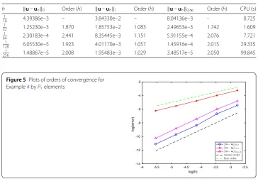
Example4 As the last testing case, we consider a problem on domainΩ= [0, 1]2with an interface of flower petal, whose parametric form is given as (cf. Example 9 of Ref. [9]):
x(θ) =a+bcos(mθ)sin(nθ)cos(θ),
Table 4 Convergence order with respect tohof the stabilized method for Example4with coefficient functions
h u–uh0 Order (h) u–uh1 Order (h) u–uh0,∞ Order (h) CPU (s) 1
16 4.39386e–3 – 3.84330e–2 – 8.04136e–3 - 0.725
1
32 1.25230e–3 1.870 1.85753e–2 1.083 2.49653e–3 1.742 1.609
1
64 2.30183e–4 2.441 8.35445e–3 1.151 5.91155e–4 2.076 7.721
1
128 6.05530e–5 1.923 4.01170e–3 1.057 1.45916e–4 2.015 29.335
1
256 1.48867e–5 2.008 1.95483e–3 1.029 3.48517e–5 2.050 99.845
Figure 5Plots of orders of convergence for Example4byP1elements
Here we takea= 0.50012563,b= 0.250012563,m= 0, andn= 10. The coefficient function and the analytical solution are chosen as
ν1= (xy+ 2)/5, ν2=
x2–y2+ 3/7;
u1=x+y+ 1, u2=sin(x+y) +cos(x+y) + 1.
For this testing case, the error inL2,H1andL∞norms and corresponding CPU time are listed in Table4. Meanwhile, the numerical orders of convergence with respect to decreas-ing mesh sizehare plotted in Fig.5. We can observe how the optimal convergence results emerge.
6 Conclusions
In this paper we have proposed a stabilized coupled algorithm for the elliptic interface problem. The main contribution of the present work is the analysis of the optimal error estimates for the present algorithm. Due to its simplicity of scheme construction, it can be generalized to even higher-order accuracy schemes for more complicated interfaces related to time and space. Several numerical experiments have also been conducted to demonstrate the computational stability and effectiveness of the present algorithm. In the next step we will be concerned with some moving interface problems for more compli-cated fluid models.
Funding
Availability of data and materials
Please contact the author for data requests.
Competing interests
The authors declare that they have no competing interests.
Authors’ contributions
The authors declare that the study was realized in collaboration with equal responsibility. All authors read and approved the final manuscript.
Author details
1College of Science, Donghua University, Shanghai, China.2Institute for Nonlinear Sciences, Donghua University,
Shanghai, China.3College of Science, Harbin Institute of Technology, Shenzhen, China.4College of Mathematics and
Systems Science, Xinjiang University, Urumqi, China.5Institute of mathematics and Physics, Xinjiang University, Urumqi,
China.
Publisher’s Note
Springer Nature remains neutral with regard to jurisdictional claims in published maps and institutional affiliations.
Received: 3 May 2019 Accepted: 5 September 2019 References
1. Peskin, C.S.: Numerical analysis of blood flow in heart. J. Comput. Phys.25, 220–252 (1977)
2. Leveque, R.J., Li, Z.: The immersed interface method for elliptic equations with discontinuous coefficients and singular sources. SIAM J. Numer. Anal.31, 1019–1044 (1994)
3. Berthelsen, P.A.: A decomposed immersed interface method for variable coefficient elliptic equations with non-smooth and discontinuous solutions. J. Comput. Phys.197, 364–386 (2004)
4. Yu, S., Zhou, Y., Wei, G.: Matched interface and boundary (MIB) method for elliptic problems with sharp-edged interfaces. J. Comput. Phys.224, 729–756 (2007)
5. Zhao, J., Hou, Y., Li, Y.: Immersed interface method for elliptic equations based on a piecewise second order polynomial. Comput. Math. Appl.63, 957–965 (2012)
6. Xia, J., Li, Z., Ye, X.: Effective matrix-free preconditioning for the augmented immersed interface method. J. Comput. Phys.303, 295–312 (2015)
7. Li, Z., Lin, T., Lin, Y., Rogers, R.: An immersed finite element space and its approximation capability. Numer. Methods Partial Differ. Equ.20, 338–367 (2004)
8. Gong, Y., Li, B., Li, Z.: Immersed-interface finite-element methods for elliptic interface problems with non-homogeneous jump conditions. SIAM J. Numer. Anal.46, 472–495 (2008)
9. Mu, L., Wang, J., Ye, X., Zhao, S.: A new weak Galerkin finite element method for elliptic interface problems. J. Comput. Phys.325, 157–173 (2016)
10. Fries, T.P., Belytschko, T.: The extended-generalized finite element method-an overview of the method and its applications. Int. J. Numer. Methods Eng.84, 253–304 (2010)
11. Zhao, J., Hou, Y., Song, L.: Modified intrinsic extended finite element method for elliptic equation with interfaces. J. Eng. Math.97, 1–13 (2016)
12. Babuška, I., Banerjee, U.: Stable generalized finite element method (SGFEM). Comput. Methods Appl. Mech. Eng.201, 91–111 (2012)
13. Hou, S., Song, P., Wang, L., Zhao, H.: A weak formulation for solving elliptic interface problems without body fitted grid. J. Comput. Phys.249, 80–95 (2013)
14. Hou, S., Wang, L., Shi, L.: An improved non-traditional finite element formulation for solving the elliptic interface problems. Comput. Math. Appl.73, 374–384 (2017)
15. Bernardi, C., Verfürth, R.: Adaptive finite element methods for elliptic equations with non-smooth coefficients. Numer. Math.85, 579–608 (2000)
16. Morin, P., Nochetto, R.H., Siebert, K.G.: Convergence of adaptive finite element methods. SIAM Rev.44, 631–658 (2002) 17. Cai, Z., Zhang, S.: Recovery-based error estimator for interface problems: conforming linear elements. SIAM J. Numer.
Anal.47, 2132–2156 (2009)
18. Chen, Z., Zou, J.: Finite element methods and their convergence for elliptic and parabolic interface problems. Numer. Math.79, 457–492 (1998)
19. Yu, J., Shi, F., Zheng, H.: Local and parallel finite element method based on the partition of unity for the Stokes problem. SIAM J. Sci. Comput.36, 547–567 (2014)
20. Zheng, H., Shi, F., Hou, Y., Zhao, J., Cao, Y., Zhao, R.: A new local and parallel finite element algorithm based on the partition of unity. J. Math. Anal. Appl.435, 1–19 (2016)
21. Shan, L., Zheng, H.: Partitioned time stepping method for fully evolutionary Stokes–Darcy flow with Beavers–Joseph interface conditions. SIAM J. Numer. Anal.51, 813–839 (2013)
22. Hou, Y.: Optimal error estimates of a decoupled scheme based on two-grid finite element for mixed Stokes–Darcy model. Appl. Math. Lett.57, 90–96 (2016)
23. Zhang, Y., Hou, Y., Shan, L.: Stability and convergence analysis of a decoupled algorithm for a fluid-fluid interaction problem. SIAM J. Numer. Anal.54, 2833–2867 (2016)
24. Layton, W., Schieweck, F., Yotov, I.: Coupling fluid flow with porous media flow. SIAM J. Numer. Anal.40, 2195–2218 (2002)
25. Adams, R.A.: Sobolev Spaces. Academic Press, New York (1975)
27. Galdi, G.P.: An Introduction to the Mathematical Theory of the Navier–Stokes Equations: Steady-State Problems. Springer, Berlin (2011)
28. Hecht, F., Le Hyaric, A., Ohtsuka, K., Pironneau, O.: Freefem++, Finite elements software.http://www.freefem.org/ff++/