Index Terms Machine Learning, Analysis of Algorithms, Spam Filtering, Naïve Bayes Algorithm, Multinomial Naive Bayes,

(1)

http://dx.doi.org/10.29322/IJSRP.9.11.2019.p9515

www.ijsrp.org

Text Analysis: Naïve Bayes Algorithm using Python

JupyterLab

A. S. Thanuja Nishadi

Faculty of Graduate Studies, University of Colombo, Sri Lanka

[email protected]

DOI: 10.29322/IJSRP.9.11.2019.p9515

Abstract-The use of mobile phones has skyrocketed during the last decade hence it has generated bulk of junk messages. However, emerging machine learning algorithms are one such solutions which are used to detect and filter spam messages recently. Naïve Bayes is a powerful yet simple classification machine learning algorithm which used in predictive modelling. Thus, Naïve Bayes categorize as four forms of its implementations; however, Multinomial Naïve Bayes is used in this study. Further, it has pre-processed the data using bag – of words (BoW) using tokenizing data with Naïve Bayes algorithm. This study will explore the process of spam filtering using Naïve Bayes classifier and further predict the classification of new text as ham or spam. In addition to that, the data analysis is carried out in Python-Jupyter Lab which is the next-generation open source web-based user interface.

Index Terms—Machine Learning, Analysis of Algorithms, Spam Filtering, Naïve Bayes Algorithm, Multinomial Naive Bayes, Classification Algorithm, Bag- Of- Words

I. INTRODUCTION

he volumes of Short Messages (SMS) are growing fast due to its features of rapidness, effectiveness and low cost. However, unsolicited or unwanted text messages generate huge threats for both individuals and organizations in numerous ways. The Text Retrieval Conference (TREC) defines the term ‘spam’ as an unsolicited, unwanted messages that was sent indiscriminately(Cormack,2008). Further, the spams are usually unsolicited and also being a carrier of malware including advertisements, fraud, phishing messages, promotions etc. Many people suffer from spam messages hence its annoyance to individuals and also considered as less reliable sources. Further, spams generate loss of productivity, misuse of data, storage and bandwidth, spread of viruses and ultimately financial loss for the organizations [Wang, 2013).

Naïve Bayes is the simplest probabilistic classifier in machine learning which used in predictive modelling. The predicator variables in the Naïve Bayes are conditionally independent of other features. Further, Naïve Bayes classifier work with correlating with tokens and calculate the probability using Bayes’ Theorem to predict the spam non-spam occurrences. Moreover, it has used bag of words feature which commonly used in text classification to identify spam messages. Although, this algorithm is simple in nature, this often used in more sophisticated activities. This study will explore the process of spam filtering using Naïve Bayes classifier and further predict the classification of new text as ham or spam.

II. MACHINE LEARNING ALGORITHMS

Machine learning technologies are becoming trends in almost every filed of technological activities. Basically, machine learning is an application of artificial intelligence (AI) that provides systems the ability to automatically learn and improve from experience without being explicitly programmed (Leimbach, 1994). Further, the process of learning begins by using collection of data or observation then searching patterns of gathered data and finally aiming for decision making (Edgar & Manz, 2017). Therefore, the aim of the machine learning is to learn things automatically by computers without human intervention.

All the machine learning algorithms are often categorized into four different types including supervised, unsupervised, semi-supervised and reinforcement (Omar, et. al, 2013).

Supervised Learning: This is used in the situations of dataset which consists with a target or outcome variable (dependent variable – DV) which can be predicted from a given set of predicators (independent variables – IVs) (F.Y.O et. al, 2017). Further, the goal of this is to predict the output for the new data once the algorithm identifies the known data. In addition to that, supervised learning algorithms has two further processes such as classification and regression. The most widely supervised learning algorithms are Linear Regression, Logistic Regression, random forest, gradient boosted trees, support vector machine (SVM), neural networks, decision trees, Naïve Bayes and nearest neighbor (Ghorbani, et. al, 2015). In classification algorithm, incoming or new data is labeled based on the past samples of data and algorithms are trained to recognize the certain types of objects then classify accordingly. This is

(2)

www.ijsrp.org

goal of this model is to detect the underline structure or distribution the data set through learning more about the data (Dy & Brodley, 2004). Further, this has grouped into two segments due to the complexity of the logic including clustering and association (Khanum, 2015). Discovering the inherent groups in the data set is performed in the clustering process. However, association rule is used to describe the large proportions of data in the association process. The most popular examples of unsupervised learning algorithms are K-Means clustering, t-SNE (t-Distributed Stochastic Neighbor Embedding and PCA (Principal Component Analysis and Association Rule (Dy & Brodley, 2004).

Semi-supervised Learning: These algorithms represent a middle ground between supervised and unsupervised features. However, some models combine the features of both aspects (Prakash & Nithya, 2014). This is basically assigns the situations where the dataset consists with both labeled and unlabeled data for training.

Reinforcement Learning: This interacts with its environment by producing actions and discovers errors or rewards. The decisions are taken sequentially i. e. outcome depends on the state of the current input and the next input depends on the output of the previous input (Mao, et. al, 2016).

III. NAÏVE BAYES CLASSIFIER

Naïve Bayes classifier is a supervised learning technique which is used for classification tasks. Further, the classifier is mainly used in analytical and predictive problems when the dimensionality of the inputs is high. Despite the simplicity, this is often used in more sophisticated classification methods (Dada, et. al, 2019).

Bayes Theorem: The classifier in Naïve Bayes is based on the Bayes theorem.

𝑃(𝐴|𝐵) =𝑃(𝐵|𝐴)𝑃(𝐴)

𝑃(𝐵)

P(A|B)=P(B1|A)× P(B2|A)× P(B3|A)×…………. P(Bn|A)× P(A)

According to Bayes Theorem, it can be found the probability of A happening, when B has occurred. In this formula, B is the evidence and A is the hypothesis. Further, the presence of one particular feature does not affect to the other hence that is referred as ‘naïve’. In this formula,

𝑃(𝐴|𝐵) is the posterior probability of class (A, target) given predictor (B, attributes)

𝑃(𝐴) is class prior probability

𝑃(𝐵|𝐴) is the likelyhodd of the probability of predictor in a given class

𝑃(𝐵) is the prior probability of predictor

IV. SAMPLE DATA SET

The dataset is received from https://www.kaggle.com in order to validate Naïve Bayes classification algorithm using Spam/Ham classification from SMS dataset.

Posterior Probability

Likelihood

Class Prior Probability

(3)

www.ijsrp.org

V. DATA ANALYSIS

[image:3.595.78.543.279.516.2]

In order to build the Naïve Bayes model, the following stages were carried out. The major stages were identified as data acquisition, data pre-processing, splitting the data as training and testing, model creation and model evaluation.

Figure 1: Steps of Machine Learning Process

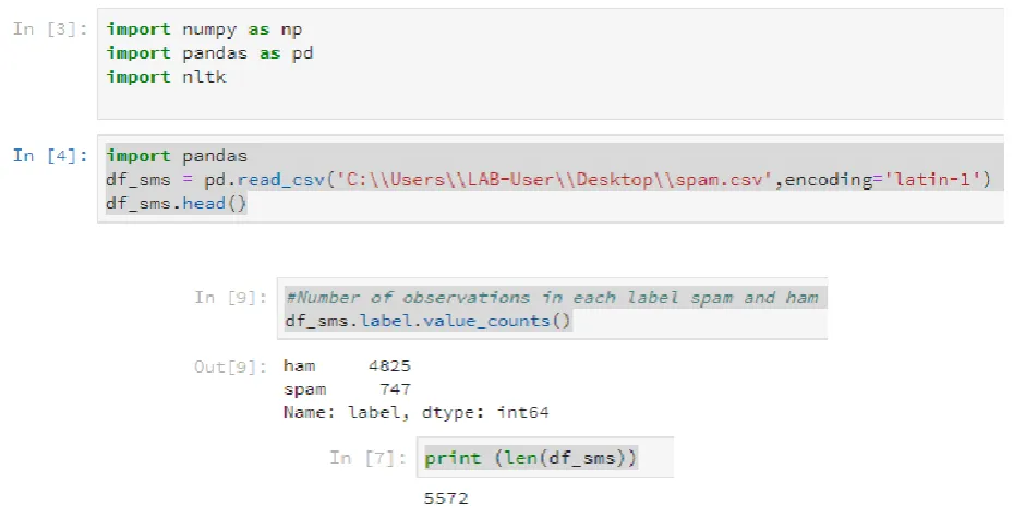
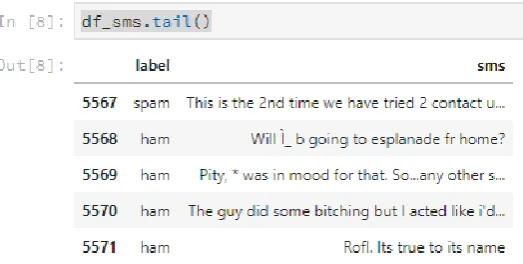
a) Data Acquisition: The sample data set (spam.csv) is loaded to Python-Jupiter lab. The dataset contains messages which composed by two columns (v1: label including ham or spam and v2: SMS which contains raw text). Further, the data set is comprised of total 5572 observations of messages. It includes 4825 ham messages and 747 spam messages.

b) Data Pre-Processing: Data pre-processing is the process of cleaning the data before applying the algorithms. The data set includes an additional unnamed column. Therefore, it has dropped the unwanted columns Unnamed:2, Unnamed: 3 and Unnamed:4 using coding. The following code indicates how it removes the additional column and the label with SMS text content of sample raw data using head and tail function. Further, it has used bag-of-words methods in data cleaning process.

Data Aquisition

Data Pre-Processing

Split Training and Testing

Data

Model Creation

(4)

www.ijsrp.org

Further, following descriptive information indicates how the label, message and length of each message.

[image:4.595.168.430.58.190.2]

Implementation of Bag-of-Words (BoW): BoW is a very common feature extraction procedure in Natural Language Processing (Belinkov & Glass, 2019). It is highly required to check whether the text document is best fit as a feature vector prior to apply machine learning algorithms.

Figure 2: Steps of Bag of Words (BoW)

All these rows of data converted into tokens or individual words. Vocabulary is the collection of unique words. Further, those tokens were observed and found the frequency of each token. Any order or structure of the words in the document (bag of words) is discarded. However, this is used when the known words are in the document only.

Tokenization: The text corpus is split into individual elements. Further, it has converted all strings into lower cases in this stage.

The above outcome shows how it has converted the messages of text into lower cases. Then, it has removed all the punctuation in the same tokenization stage.

Gather

Text Data

Clean

Text

Tokenize

vocabulary

(5)

www.ijsrp.org

The above code with the outcome shows how it has removed the punctuations in the text. In addition, that, the below code indicate how it used convert sentences into words or tokenization.

Then, it has found the count of occurrence of each token using Term Frequency – Inverse Document Frequency (TF – IDF) technique. TF is the measure frequency of a word in a data set whereas IDF measures the rank of the specific word.

Term Frequency (TF): This is a scoring of the frequency of the word in the current document.

𝑇𝐹(𝑡) =𝑁𝑢𝑚𝑏𝑒𝑟 𝑜𝑓 𝑡𝑖𝑚𝑒𝑠 𝑡ℎ𝑒 𝑤𝑜𝑟𝑑 (𝑡) 𝑜𝑐𝑐𝑢𝑟𝑠 𝑖𝑛 𝑡ℎ𝑒 𝑡𝑒𝑥𝑡

𝑇𝑜𝑡𝑎𝑙 𝑛𝑢𝑚𝑏𝑒𝑟 𝑜𝑓 𝑤𝑜𝑟𝑑𝑠 𝑖𝑛 𝑡ℎ𝑒 𝑡𝑒𝑥𝑡

Inverse Document Frequency (IDF): This is a method of scoring how rare the word is across the document.

𝐼𝐷𝐹(𝑡) = 𝑇𝑜𝑡𝑎𝑙 𝑛𝑢𝑚𝑏𝑒𝑟 𝑜𝑓 𝑑𝑜𝑐𝑢𝑚𝑒𝑛𝑡𝑠

𝑁𝑢𝑚𝑏𝑒𝑟 𝑜𝑓 𝑑𝑜𝑐𝑢𝑚𝑒𝑛𝑡𝑠 𝑤𝑖𝑡ℎ 𝑡𝑒𝑟𝑚 𝑡 𝑖𝑛 𝑖𝑡

(6)

www.ijsrp.org

The mapping from textual data to vector is referred as feature extraction. Then, the CountVectonizer() method is used to data cleaning process. Further, the steps of cleaning include converting all data to lower cases and removing all punctuation marks in the data set. Steps followed in CountVectorizer as follows.

 Create an instance of the CountVeconizer class

 Call the fit () function to find the vocabulary from one or more documents

 Call the transform () function on one or more documents as it needed to encoded each as a vector

c) Splitting Dataset in Training and Testing Sets

(7)

www.ijsrp.org

Then, the data set needed to convert into matrix using CountVectonizer(). Further, it is required to fit the training data (x_train) into CountVectonizer() and receive the matrix. Furthermore, transforming testing data (x_test) to return the matrix.

d) Model Creation: Multinomial Naive Bayes Implementation

Naïve Bayes consists with four forms of its implementations such as Gaussian, Multinomial, Complement and Bernoulli Naïve Bayes (Rennie, et. al, 2003). The Multinomial Naïve Bayes has been used in this study due to the classification of discrete features such as word counts. It takes integer word counts as inputs. However, Gaussian is used for continuous data as inputs whereas complement classifier estimates parameters of a category. But, Bernoulli assumes the distribution of probability as Bernullian.

Therefore, it has imported MulinomialNB Classifier in training data set using fit ().

According to the code snippets, it can clearly be seen that the algorithm has been trained using the training data set. Further, predictions on the test data can be processed using predict ().

e) Model Evaluation

Predictions are done using test data. Further, accuracy of the predictions is checked in this stage.

(8)

www.ijsrp.org

With considering the above output data, accuracy score of data set is 98%. Further, it has indicated as 2 messages as spams and other 98 of messages as non-spams in a sample of 100 messages. It has further used F1 score to evaluate the weighted average of the precision and recall scores. This value mainly ranges between 0 and 1. As this model receives all four matrices close to 1 this fits with the model best.

VI. CONCLUSION

The study covers how it detected the spam and non-spam messages using Naïve Bayes algorithm. This algorithm allows to handle large number of features i. e. words. Thus, Naïve Bayes support for handling large number words easily.

Further, the data set followed set of processes of machine learning in order to build the model. The data set acquired from the kaggle site and performed pre-processing using many methods including bag-of-words. Then, split the data into train and test model. Furthermore, it has built the model and evaluated. The accuracy of the model is tested using accuracy score, precision score, recall score and F1 score.

REFERENCES

[1] Belinkov, Y. and Glass, J. (2019). Analysis Methods in Neural Language Processing: A Survey. Transactions of the Association for Computational Linguistics, 7, pp.49-72.

[2] Cormack, G. (2008). Email Spam Filtering: A Systematic Review. Foundations and Trends® in Information Retrieval, 1(4), pp.335-455, DOI 10.1561/1500000006.

[3] Dada, E., Bassi, J., Chiroma, H., Abdulhamid, S., Adetunmbi, A. and Ajibuwa, O. (2019). Machine learning for email spam filtering: review, approaches and open research problems. Heliyon, 5(6), p. e01802.

[4] Dy, J.G and Broadley, C.E. (2004), Feature Selection for Unsupervised Learning, Journal of Machine Learning Research, 845–889. Available: http://www.jmlr.org/papers/volume5/dy04a/dy04a.pdf

[5] Edgar, T.W., Manz, D. O. (2017), Using Data Mining and Machine Learning Methods for Cyber Security Intrusion Detection. (2017). International Journal of

Recent Trends in Engineering and Research, 3(4), pp.109-111.

[6] F.Y, O., J.E.T, A., O, A., J. O, H., O, O. and J, A. (2017). Supervised Machine Learning Algorithms: Classification and Comparison. International Journal of

Computer Trends and Technology, 48(3), pp.128-138.

[7] Ghorbani, A., Steinhilber, G., Markus, D. and Maas, U. (2015). A PDF projection method: A pressure algorithm for stand-alone transported PDFs. Combustion

Theory and Modelling, 19(2), pp.188-222.

[8] Khanum, M., Mahboob, T., Imtiaz, W., Abdul Ghafoor, H. and Sehar, R. (2015). A Survey on Unsupervised Machine Learning Algorithms for Automation, Classification and Maintenance. International Journal of Computer Applications, 119(13), pp.34-39.

[9] Leimbach, M. (1994). Expert system model coupling within the framework of an ecological advisory system. Ecological Modelling, 75-76, pp.589-600.

[10] Mao, H., Alizadeh, M., Menache, I. and Kandula, S. (2016), Resource Management with Deep Reinforcement Learning. In ACM Workshop on Hot Topics in Networks.

[11] Prakash, V. and Nithya, D. (2014). A Survey On Semi-Supervised Learning Techniques. International Journal of Computer Trends and Technology, 8(1), pp.29.

[12] Omar, S., Ngadi, A. and H. Jebur, H. (2013). Machine Learning Techniques for Anomaly Detection: An Overview. International Journal of Computer Applications, 79(2), pp.33-41.

[13] Rennie, J. D., Shih, L., Teevan, J., & Karger, D. R. (2003). Tackling the poor assumptions of naive Bayes text classifiers. In ICML (Vol. 3, pp. 616-623).