Simplification of correspondence analysis for more precise calculation which one qualitative variables is two categorical data

(1)

SIMPLIFICATION OF CORRESPONDENCE ANALYSIS FOR MORE

PRECISE CALCULATION WHICH ONE QUALITATIVE VARIABLES

IS TWO CATEGORICAL DATA

I. Ginanjar

1

, U. S. Pasaribu

2

and A. Barra

2

1

Departement of Statistics, Universitas Padjadjaran, Indonesia

2

Departement of Mathematics, Institut Teknologi Bandung, Indonesia E-Mail: [email protected]

ABSTRACT

The calculations of correspondence analysis (CA) are using the long stages matrix operations, so that through many times rounding process, and the eigenvalues obtained by numerical process. The CA is often using standard residual matrix to calculate the singular value decomposition (SVD), this paper proves that 0 is a singular value of standard residual matrix. Based on that, this paper introduce simplification of correspondence analysis (SoCA) of 2 × J contingency table where J = 2, 3, 4, , where obtain the simpler and more precise calculation, because it managed to minimize rounding process, also does not use the numerical process, with use standardized residuals matrix as a matrix to calculate the SVD, it is very useful for data mining techniques.

Keywords: correspondence analysis, singular value decomposition, simplification, correspondence analysis, data mining. 1. INTRODUCTION

Tufféry [1] elucidate that “the most relevant fields of data mining are those where large volumes of data have to be analyzed, sometimes with the aim of rapid decision making”. Data mining is a set of methods and techniques for exploring and analyzing data sets, by automatic or semi-automatic way, to find certain provisions of the unknown or hidden, and association or trends in the data set, the outputs specifically provide useful information while reducing the quantity of data. Data mining Data mining techniques was using the inferential statistics and ‘conventional’ data analysis including factor analysis, clustering analysis, discriminant analysis, correspondence analysis (CA), etc. Data mining analysis for two qualitative variables often use CA.

CA was first discovered and developed in the 1960s by Jean-Paul Benzécri and friends in France [2]. This analysis is defined as the mapping technique of a contingency table in an optimal small-dimensional vector space. This analysis is also used to grouping the categories of rows and columns from the contingency table.

CA has been applied in various fields of science, including Education, Economics, Safety, Medical, and others. Zhibo et al. [3] analyzed and compared the competitive power of steel industry of 30 provinces in China, with data containing 16 economic indicators to reflect each province’s business conditions of steel industry. Lu et al. [4] investigated the associations between fatality levels and influence factors that involve place, cause, time of day, month, year and province. Zalewska et al. [5] described the relationship between asthma, region, and age, from Epidemiology of Allergy in Poland (ECAP) data survey in years 2006-2008.

The improvement study of CA performed by: Beh [6] introduced the Elliptical confidence regions for

CA, so the quality of the correspondence plot configuration is better, because it involves the cumulative percentage of eigenvalues of the times more than the dimensions used. Takagi and Yadohisa [7] introduced the CA based on the interval algebra, so that the calculation method of CA performed contingency table with shaped cells intervals. Beh [8] introduced the CA using the adjusted residuals so that data map can show the cross-tabulation of data variability.

The calculations of CA are using matrix operations with the long stages. That through many times rounding process, it also the eigenvalues obtained by numerical process, so that the values obtained are less precise. The principal coordinates estimate are use standardized residuals matrix, which is Greenacre in 2011 [9] showed that this matrix can position an outlier in the CA map.

This paper proposed to perform mathematical analysis of CA with one’s qualitative variables is two categorical data, to obtain the matrix model calculation method which is simpler and more precise (to minimize rounding process, also does not use numerical process and called simplification of correspondence analysis (SoCA). Ginanjar et al [10] has published the application of SoCA in 2014, while this paper writes more detailed theory of SoCA.

(2)

(Section 6) with a brief discussion of the procedure and some possible avenues for further research.

2. CORRESPONDENT ANALYSIS (CA)

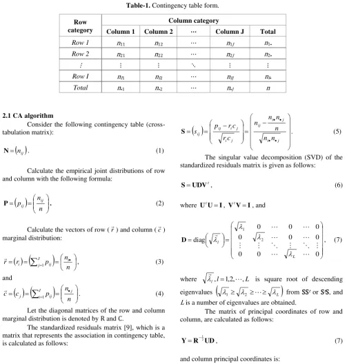
First at all, we construct a contingency table. This table is a cross-tabulation of the two categories (variables). The first category variables is the row category and the second variables is the column category, see Table-1.

Table-1 gives a IJ contingency table, where the first variable has I row categories, and the second variable has J column categories. Suppose nij is the numbers of

individuals in category i on the first variable and category j

[image:2.595.47.551.233.761.2]

in the second variable, and the total of each row isni• and the total of column is n•j, where i = 1, 2, , I and j = 1, 2, , J.ni• and n•j are called marginal for first variable with the category i and second variable with the category j, respectively. The grand total is the total number of individuals which is denoted by n.

Table-1. Contingency table form. Row

category

Column category

Column 1 Column 2 Column J Total

Row 1 n11 n12 n1J n1•

Row 2 n21 n22 n2J n2•

⋱

Row I nI1 nI2 nIJ nI•

Total n•1 n•2 n•J n

2.1 CA algorithm

Consider the following contingency table (cross-tabulation matrix):

 

nij



N . (1)

Calculate the empirical joint distributions of row and column with the following formula:

 

_

      

n n pij ij

P . (2)

Calculate the vectors of row (r) and column (c) marginal distribution:

 







      

 





n_n

p r

r J i

j ij

i 1



, (3) and

 





_

      

 





n n p c

c j _iI1 ij j



. (4) Let the diagonal matrices of the row and column marginal distribution is denoted by R and C.

The standardized residuals matrix [9], which is a matrix that represents the association in contingency table, is calculated as follows:

 

   

 

   

 

      

 

 _

 

 

j i

j i ij

j i

j i ij ij

n n

n n n n

c r

c r p s

S . (5)

The singular value decomposition (SVD) of the standardized residuals matrix is given as follows:

t UDV

S , (6)

where UtUI, VtVI, and

   

 

   

 

       

0 0

0

0 0

0

0 0

0

diag 2

1

 

     

 



L l

 

D , (7)

where l,l 1,2,,L

 

 is square root of descending eigenvalues



1 2  L



from SSt or StS, and

L is a number of eigenvalues are obtained.

The matrix of principal coordinates of row and column, are calculated as follows:

UD R

Y 2

1



 , (7)

(3)

t

VD C

Z 2

1



 , (8)

respectively.

The first two columns of the principal coordinates of row and column are the coordinates to build the two-dimensional map.

3. MATHEMATICAL ANALYSIS (CA) 3.1 Matrix for calculates the CA eigenvalues

Standard residual matrix can be calculated directly from the elements of cross-tabulation matrix (Equation (5)). SVD calculation begins by calculating the eigenvalues of the matrix product SSt_or_St_S_{. Let}_I_<_J_then

the size of the matrix SSt_{< S}t_S_{, thereby calculating}

eigenvalues of SSt_will_{be simplified.}

Lemma 1

If the size of a matrix N is I J (Equation (1)), and SSt_{= A}_{, then the elements of}_A_is

    

  







_  

 



J j

k i j

kj ij

k i ik

n n n n

n n

a 1 ₁ , (9)

where i and k = , , ,I. Proof:

 





_

_



 J

j ij kj ik s s

a ₁

A

with the result that





 

 J

j

j k

j k kj

j i

j i ij ik

c r

c r p

c r

c r p

a ₁

k i J

j j

kj ij

k i

r r c

p p

r

r 

   

  

 1



_₁

based equations (2) and (3), so,

n n n n

n n

n n n n

a J_j i k

j kj ij

k i ik

  

 



    

 

   

 





1

    

  







_  

 



J j

k i j

kj ij

k

i n

n n n

n n

n

n 1

1

. ∎

Lemma 1 is a formula to calculate SSt_{which is} simpler and more precise, because each element of the matrix is calculated directly from the elements of the

contingency Table. The variable often consists of two categories (I = 2), e.g. gender, yes or no, and others. Based on that, this paper formulates the lemma of SSt_for₂ × J contingency table.

Lemma 2

If the size of a matrix N is 2 × J (Equation (1)), and SSt_{= A}_{, then the elements of}_A_{is obtained}

21 1 2 12

1 2 22

1 2

11 a

n n a

 



 __ __

 . (10)

Proof

Let 

   2

2 1

1 n

n n n





 

   



2 2

2 1

1 1 2 n n

n n n n J

j j j









_

  

 

 

 _ _

    

 





2 2

2 1 1

1 1 2

1 n n

n n n n

n

n J_j j

J

j j j J

j j

    

  

    

  

 

    

  







  

  

  

J j

j j J

j j j

n n n n

n n n n n n n

n 1

2 2 2 2 2

1 2 1

2 1 2 1 1

1 1

,

byLemma 1 is obtained 22 1 2

11 a

n n a

 

 .

Let 

   2

2 1

1 n

n n

n

n n n n n n

n

J

j j _ _

  

 _ _ 



1 2

2 1 2

1 1





n n

n n n n n

n n n

n j j

j j J j j

    



 

 



2 2 1 1 2 1

2 1 1 1 2

1

n n

n n n n n

n n n

n n n n

J j

j j j

      

 

  

 



2 2 1 1 2 1 1

2 1

2 1 1 2

1

    

  

 



_

_

 

J j

j j

n n

n

n n

n 1

2 2 1 2 1

2

1

(4)

    

  



 _ _

  

 





n n n

n J

j j

j

j 1 2

1 2 1 2

1 2

1 1

    

  

 





_ 

 



 J

j j j

n n

n n n

1

2 1 2 1

1 2

1 1

by Lemma 1 is obtained, 11 2 1 12 2 1

a n n a n n

  

 _

21 1 2 12 1 2

11 a

n n a

  

 __

 

then,

21 1 2 12

1 2 22

1 2

11 a

n n a

 



 __ __

 . ∎

3.2 Eigenvalues and orthonormal eigenvector The equations for calculating eigenvalues are

0 )

det(



ISSt  . (11) The calculation of SSt _eigenvalues _has

uniqueness. SSt_{is a real symmetric matrix that has the}

following properties: 1) is positive semidefinite, 2) is always diagonalizable, 3) has orthogonal eigenvectors, and 4) has only real eigenvalues. Other than that 0 is eigenvalue of SSt_{, it is proved in Theorem 1.}

Theorem 1

If the size of a matrix N is I × J (Equation (1)), and SSt_{= A}_{, then 0 is eigenvalue of}_A_.

Proof

Let w



r r  rI





, , ₂

1

 with 1

1 1



 I

i r .

Then

  

 

  

     

 

  

 

    

   



 

I i i iJ I i i i

I IJ J

I t

s r

r r

s s

w

1

1 1

1

1 11

 

 

 

 

S









     

 

     

 

 



     

 

     

 

 





 

I i i J I

i iJ J

I i i I

i i

I i

J J i iJ I i

i i

c r p

c

c r p

c

c c r p

1 1

1 1 1

1 1

1 1 1

1 1











0

1 1

1 1 1 1

1 

 

     

 

     

 

 





  I i i J J J

I i i

r c c c

so, we obtained

 

0 0

   



  

 SS SS S

Aw t w tw , has a non-trivial solution. Then 0 is eigenvalue of A.∎

The eigenvalues calculation involves the calculation of polynomial roots, which has been obtained through numerical process. The eigenvalues calculation of the matrix size 2 × 2 can be performed using mathematical analysis, so the eigenvalues are obtained more precise. If the size of a matrix SSt_is_{2 × 2}_{, with}

Lemma1, Lemma 2, and Theorem 1, then the eigenvalues can be calculated directly from the elements of the contingency table, which is described in Lemma 3. Lemma 3

If the size of a matrix N is 2 × J (Equation (1)), and SSt_{= A}_{, then the first eigenvalues (}λ_{1) corresponding}

to A is _

  

  









 



J j

j j

n n

n

1

2 1 2 1

2 1

, and the second eigenvalues (λ2) corresponding to A is 0.

Proof

From Theorem 1 than the result that λ2 =0. From Lemma 2 be discovered 11

2 1

22 a

n n a

 

 , than the result that:

     

  

   

  



2 1 11 11 2 1 11 22 11

1 tr( ) 1

n n a a n n a a a A 

with Lemma 1 than the result that:

     

     

  

 

  





2

1 1

2 1 2 1

1

1 1

1

n n

n J

j j j 

    

  







_ 

 

 J j

j j

n n n n n

n n

1

2 1 2 1 2

1 1

 . ∎

As a result of the Lemma 3 it can be seen that for the size of a matrix N is 2 × J, will be obtained 1-dimensional principal coordinate, with 100% contribution ratio.

The equations for calculating eigenvector are





* 0

 

 SSt u

I

(5)

If the size of a matrix SSt_is_{2 × 2}_{, and}λ_{is the}

eigenvalues of SSt_{, then with Lemma 2, and Theorem 1 the}

orthonormal eigenvectors can be calculated. The orthonormal eigenvectors are the columns for the matrix U

(Equation (6)), which can be calculated directly from the elements of the contingency table, and written on Lemma 4. Lemma 4

If the size of a matrix N is 2 × J (Equation (1)), and SSt_{= A}_{, then the orthonormal eigenvectors from}_A_are





_            2 1 1 2 2 1 1 n n n n n u

u  .

Proof

With Lemma 1, Theorem 1, and the Equation (12) are obtained

0 * 12 * 11 11 2 1 11 2 1 11 2 1 11 _                                u u a n n a n n a n n a   ,

let the eigenvector for 11 2 1 11 1 a n n a    

 is:

0 * 12 * 11 11 11 2 1 11 2 1 11 2 1                                 u u a a n n a n n a n n

by using elementary row operations, so obtained

                              1 2 * 12 * 11 * 12 * 11 1 2 0 0 0 0 1 n n u u u u n n .

let u12* t, so the eigenvector is

                    t n n t u u 1 2 * 12 * 11

The orthonormal eigenvector is eigenvector vector with length is 1, so the orthonormal eigenvector for λ1, is eigenvector for λ1 which each element is divided by

   _ _           1 2 2 1 2 * 1 n n t t n n t

u ,

so the orthonormal eigenvector for λ1 is:

                                1 2 1 1 2 12 11 1 n n n n t n t n n t u u ,

and the eigenvector for λ2 =0 is:

0 * 22 * 21 11 2 1 11 2 1 11 2 1 11 _                              u u a n n a n n a n n a

by using elementary row operations, so obtained

                              2 1 * 22 * 21 * 22 * 21 2 1 0 0 0 0 1 n n u u u u n n .

Let u22* t, so the eigenvector is

                   t n n t u u 2 1 * 22 * 21 _,

the orthonormal eigenvector for λ2, is eigenvector for λ2 which each element is divided by

   _ _          2 2 2 2 1 * 2 n n t t n n t u

so the orthonormal eigenvector for λ2 is:

                               2 1 2 2 1 22 21 1 n n n n t n t n n t u u ,

then, the orthonormal eigenvectors from A are:





_            2 1 1 2 2 1 1 n n n n n u

u  . ∎

With using Equation (5), Equation (6), and Lemma 4, than the elements of the orthonormal eigenvectors

 

v1



(6)

Lemma 5

If the size of a matrix N is 2 × J (Equation (1)), and SSt_{= A}_{, then the elements of orthonormal}

eigenvectors

 

v1 

from the first eigenvalues

 

1

corresponding to St_S_is

n n n n

n n n n v

j j j j

  

 



2 1 1

2 1 1 2 1

 for j = 1, 2,

, J. Proof

Based on the SVD (Equation (6)) are obtained:

2 2 21 1 1 11

1j u vj  u vj 

s  

and

2 2 22 1 1 12

s   .

Calculate vj2 from s2j,

2 2 22 1 1 12

s  

2

2 22

1 1 12 2

j j

j

v u

v u s

 

 

,

substitution vj2 into s1j,

2 22

1 1 12 2 2 21 1 1 11 1

  



u v u s u v

u

s j j j j

 





11 22 21 12



1 2 21 22 1 1

 u u u u

s u u s

v_j j j

  



2 2 1 1



1 2 1 2 1 1

1

    

 

  

n n n n

s n n s

n

v_j j j

n s n n

s j j

1 2 1 2 1

 



  

Based on Equation (5), than the result that:

n

n n n

n n n n n n n

n n n n

v j

j j

j j j

j

1

1 2

2 2 2 1

1 1

1

 

  



 

   

 

n

n n n

n n

n n n

n n

j j

1

2 1 2

1 2 1

 

 



  

    

 

     



n

n n n n

n n

n

n j j

j j

1

2 1

1 2

2 1 2

1 2 1

 

 

 

      

  

 

n n n n

j j j

  

 



2 1 1

2 1 1 2

 . ∎

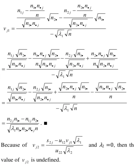
Because of

2 22

1 1 12 2 2

 

u v u s

v_j  j j and λ2 =0, then the value of vj2 is undefined.

3.3 Principal coordinates of rows and columns

The main objective of the CA is to estimate the principal coordinates, for mapping the row and column categories of a contingency table. The principal coordinates are the linear combinations vectors from each row or column category.

[image:6.595.307.541.100.388.2]

Based on Lemma 3, Lemma 4, and Lemma 5, then the author can make an equation to estimate the principal coordinates, which is simpler and more precise, which is calculated directly from the elements in contingency table. It was described in Theorem 2.

Theorem 2

If the size of a matrix N is 2 × J (Equation (1)), then the row principal coordinates Y is

    

     

  





0 0

0 0 1 1

2 1 1

2 1 2 1

 

n n n n

n

n J

j j j

Y

and the column principal coordinates Z is



1 0



 

j

z



Z where

  

 



2 1

2 1 1 2 1

n n n

n n n n z

j j j

j .

Proof

(7)

                               0 0 0 0 0 1 1 0 0 1 1 2 1 1 2 2 1    n n n n n r r Y                                       0 0 0 0 0 0 0 0 2 1 1 2 1 2 1 1 2 1     n n n n r n r n n  

                                 



0 0 0 0 2 1 1 2 2 1 1 2 1 2 1   n n n n n n n n n n n J j j j Y                        



0 0 0 0 1 2 1 1 1 1 2 1 1   n n n n n n n n n n J j j j                 





0 0

0 0 1 1 2 1 1 2 1 2 1   n n n n n n n n J j j j               





0 0

0 0 1 1 2 1 1 2 1 2 1   n n n n n n J j j j

The column principal coordinates (Equation (7)) is:

                                             0 0 0 0 0 1 0 0 0 1 0 0 0 1 1 2 1 2 2 2 2 1 1 1 2 1 1 2 1                  JJ J J J J J v v v v v v v v v c c c Z                      0 0 0 1 1 2 21 1 1 11 1 J J c v c v c v     





                      0 0 0 0 1 1 2 21 1 1 11 1 1 J J j c v c v c v z       

Z where

j j j

c v z₁ ₁ 1

          _   2 1 2 1 1 2 2 1 1 2 1 1 2 1 1 n n n n n n n nc n n n n n n n z j j j j j j j j   . ∎ 4. EXAMPLE

This section is presents an example to describe the steps of SoCA. The example is used fraud consumer data with two qualitatively random variables. The variables are Card type and Countries based on IP Address. The data are obtained from an online payment gateway company in Indonesia.

4.1 Transform two qualitative variables into a contingency table

Transform two qualitative variables (card type and IPID Country) into contingency table, so we got the data shown in Table-2.

Table-2. Contingency table: card type and IPID Country.

Card Type IPID Country

(8)

4.2 Compute the principal coordinates of rows and column

Compute the principal coordinates of rows using Theorem 2, where



2₂



1

3 3 4 3 13 5 1 0 81 54 4 2 2 2 9 1 1 1 73

120 2 2 2 2 2 2 2 2 2 2

2          



Y

   

  

0 0

0 0 1

47

73 _



   

      

  

0 0 5147 . 0

0 0 3314 . 0 0 0

0 0 1 1098 . 0

47

73 _ _



Compute the principal coordinates of columns using Theorem 2, where

8024 . 0

47 73 1

47 1 73 0 11

2 1 1

2 11 1

21  

   _

  

 

n n n

n n n n

z ,

0186 . 1

47 73 9

47 1 73 8 21

2 1 2

2 12 1

22  

   _

  

 

n n n

n n n n

z ,

8024 . 0

47 73 2

47 2 73 0 31

2 1 3

2 13 1

23  

   _

  

 

n n n

n n n n

z ,

2219 . 0

47 73 4

47 2 73 2 41

2 1 4

2 14 1

24  

   _

  

 

n n n

n n n n

z ,

1195 . 0

47 73 81

47 54 73 27 51

2 1 5

2 15 1

25  

   _

  

 

n n n

n n n n

z ,

2463 . 1

47 73 1

47 0 73 1 61

2 1 6

2 16 1

26  

   _

  

 

n n n

n n n n

z ,

4583 . 0

47 73 13

47 5 73 8 71

2 1 7

2 17 1

27  

   _

  

 

n n n

n n n n

z ,

2902 . 0

47 73 4

47 3 73 1 81

2 1 8

2 18 1

28  

   _

  

 

n n n

n n n n

z ,

8024 . 0

47 73 3

47 3 73 0 91

2 1 9

2 19 1

29  

   _

  

 

n n n

n n n n

z ,

8024 . 0

47 73 2

47 2 73 0 1

10

2 1 10

2 10 1 1 10

2  

   _

  

 

n n n

n n n n

z .

4.3 Plot the projections of data

The first two columns of the principal coordinates of rows and columns are the coordinates to make the map of SoCA where presented in Figure-1.

Figure-1. SoCA map of card type and IPID Country. Figure-1 show that most of the fraud customer from Argentina, Canada, Spain, and the USA using Visa, and most of the fraud customers from Australia and Malaysia using MasterCard. The fraud customers from Singapore and Indonesia predominant use Visa and MasterCard partly use. The fraud customer from Mexico and India predominant use MasterCard and Visa partly use.

5. DISCUSSION AND CONCLUSIONS

This paper has shown that SoCA obtains the simpler and more precise calculation method, because it managed to minimize rounding process, also does not use numerical process. The standardized residuals matrix is used for calculate the SVD, which rare objects are often positioned as outliers in CA map, which gives the impression that they are highly influential, but their low weight offsets their distant positions and reduces their effect on the results. For each N(2J) is a cross tabulation

matrix (Equation 1) where j = 1, 2, , J, will be obtained one-dimensional visualization, with the contribution ratio of 100%. The idea of SoCA of 2 × J contingency tables can be highly enlightening as to the properties of these methods. In future work we will generalize SoCA to be used for I × J contingency tables where I = 3, 4, 5 and J = 2, 3, .

ACKNOWLEDGEMENT

The authors thanks to Dr. Sapto W. Indartno, who have provided direction, correction and perfection solution for this paper, we also thank the editor. Work supported by grants BPP-DN from Indonesian directorate general of higher education.

REFERENCES

[1] S. Tufféry. 2011. Data Mining and Statistics for Decision Making. John Wiley and Sons, Ltd, United Kingdom.

[2] J.P. Benzécri. 1992. Correspondence Analysis Handbook. Marcel Dekker Inc., New York, USA. [3] R. Zhibo, L. Kai and W. Wei. 2012. The Comparative

Study of the Competitive Power of the Steel Industry

(9)

of Every Province in China Based on Correspondence Analysis Method. Physics Procedia. 25: 1671-1674. [4] S. Lu, P. Mei, J. Wang and H. Zhang. 2012. Fatality

and influence factors in high-casualty fires: A correspondence analysis. Safety Science. 50: 1019-1033.

[5] M. Zalewska, K. Furmańczyk, S. Jaworski, W. Niemiro and B. Samoliński. 2013. The Prevalence of Asthma and Declared Asthma in Poland on the Basis of ECAP Survey Using Correspondence analysis. Computational and Mathematical Methods in Medicine. 2013: 1-8.

[6] E.J. Beh. 2010. Elliptical confidence regions for simple correspondence analysis. Journal of Statistical Planning and Inference. 140: 2582-2588.

[7] I. Takagi and H. Yadohisa. 2011. Correspondence analysis for symbolic contingency tables based on interval algebra. Procedia Computer Science. 6: 352-357.

[8] J.E. Beh. 2012. Simple correspondence analysis using adjusted residuals. Journal of Statistical Planning and Inference. 142: 965-973.

[9] M. Greenacre. 2011. The Contributions of Rare Objects in Correspondence Analysis, Barcelona GSE Working Paper Series. No. 571.