ISSN Online: 2160-8849 ISSN Print: 2160-8830
Quantification of Node Wise Commodity in
Supply Chain and Its Cost Analysis
Prem Prakash Mishra1, S. S. Mishra2*, S. K. Yadav2, R. S. Singh3,Ravendra Kumar4
1Department of Mathematics, National Institute of Technology, Chumukedima, Nagaland, India 2Department of Mathematics and Statistics, Dr. RML Avadh University, Faizabad, India
3Kamla Nehru Institute of Management, Dr. APJ Abdul Kalam Technical University, Lucknow, India 4Department of Mathematics, Dr. Ram Manohar Lohia Government Degree College, Aonla, India
Abstract
In this paper, we focus on the intermediate nodes of network and quantifica-tion of level of commodity and its cost on each node because intermediate nodes have stocking capacities which we generally see in the supply chain network. The commodity is supplied from a node to node in response to the power form of demand at a particular time. Since the traffic intensity of the demand of commodity also affects the flow of the commodity in the network, hence study of flow of commodity in the network is believed to be a signifi-cant contribution in this area. Several cases of quantifying the level of com-modity in different situations as well as the cost analysis of incoming and outgoing commodity at a particular node have been thoroughly discussed in the paper. The present problem, presumably seeks to contribute to managerial decision making in supply chain network.
Keywords
Supply Chain, Traffic Intensity, Node Wise Amount of Flow and Cost Analysis
1. Introduction
A fresh attempt needs to be made to quantify the level of commodity on the nodes of supply chain network at any instant of time with a particular amount of flow. Here, we seek to characterize the nodal properties of the network which in turn helps in making the strategies for future plans about a particular node of network and gauge the degree of importance of a particular node in whole net-work. Node wise quantification commodity paves the way for obtaining the economic inflow quantity at the node as well as the total optimal cost of the
How to cite this paper: Mishra, P.P., Mi-shra, S.S., Yadav, S.K., Singh, R.S. and Ku-mar, R. (2017) Quantification of Node Wise Commodity in Supply Chain and Its Cost Analysis. American Journal of Opera-tions Research, 7, 64-82.
http://dx.doi.org/10.4236/ajor.2017.71005
Received: November 11, 2016 Accepted: January 21, 2017 Published: January 24, 2017
Copyright © 2017 by authors and Scientific Research Publishing Inc. This work is licensed under the Creative Commons Attribution International License (CC BY 4.0).
network system. In this sequence of knowledge, we wish to report some impor-tant developments which are relevant to it. Ahuja et al. [1] have combined the several techniques to produce an algorithm for non-sparse graphs with large maximum arc capacity and also discussed about the bound for the transporta-tion problems. Ahuja et al. [2] defined the flow in a network N (V, E) as a real function x V V: × →R with the three properties
1) Capacity constraints: xij≤C i j
( )
, . The flow along an edge cannot exceedits capacity, ∀i j V, ∈ .
2) Skew symmetric: xij = −xji. The flow from i to j is xij and the flow from j to i is xij.
3) Flow conservation: ij 0
j V
x
∈ =
∑
unless i = source or j = sink.The net flow to a node is zero except for the source that “produces” flow and the sink which “consumes” flow.
This paper focuses on the third condition at the intermediate nodes of the network where summation of all incoming flow and outgoing flow is zero, but in some case of the supply chain network this conservation law at instantaneous incoming and outgoing of flow does not hold good. In this situation, value of the flow is given as below at the intermediate node which appears like source or sink for short length of time that is given below, where xi is called the amount of flow. The amount of flow at th
i node is treated as variable in case of the
ran-dom network of the supply chain. During the ranran-dom alteration in incoming flow and outgoing flow of commodity at the th
i node, the amount of flow
changes with time.
To manage the fluctuation in the amount of flow at intermediate nodes re-quire storage capacity. This phenomenon provides me with the insight to meas-ure the level of commodity which will be stored during this random change in the network. In case of the information flow, we will be able to know about the level of information at particular time according to that we may solve the routing problem of information flow with performance objectives.
Consider a node in computer communication network that receives the pack-et of information from various sources and must forward them toward their un-limited destination. Generally, the node has a fixed or at least a maximum rate at which it can transmit data. Since the arrival of packet to a node will be quite random, the node will usually have some buffering capacity, allowing the node to temporarily store packets which it can forward immediately.
economic order quantity model for queued customers with normal life time of inventory flowing in supply chain. Mishra and Singh [5] worked on an economic order quantity (EOQ) model with quadratic deterioration items allowing short-ages for computing the total optimal cost. There are other several researchers Mishra and Mishra [6] investigated an inventory model for deteriorating items under cobweb phenomenon and permissible delay in payment for fuzzy envi-ronment. And Mishra et al. [7] illustrated the inventory flow in supply chain with deteriorating items for customers in queue and optimized the profit under in fuzzy environment. Jose et al. [8] have worked on the online measurement of large traffic aggregates on commodity switches such as anomaly detection and traffic engineering and also proposed a practical measurement model based on emerging open flow switches. Gill et al. [9] have compiled models of information flow through queuing network and the multi-hop flow routing dimension. They also proposed it as convex optimization problem. Thomas et al. [10] analyzed passive measurement system for network test beds. The ability to capture and process packet-level data is of intrinsic importance in network test beds that of-fer broad experimental capabilities to researchers. Since we know that commod-ity may be the energy or oil, gas, fluid etc. Narasimhan [11] and Farlow [12] worked on the Fourier’s heat conduction equation wrote that Fourier’s heat conduction equation i.e. u x t
( )
, k 22u x t( )
,t x
∂ = ∂
∂ ∂ continues to constitute the conceptual foundation on which rests the analysis of many physical, biological, and social systems. This equation of heat flow may be treated as the partial dif-ferential equation of the commodity flow which has most important role in this paper. Sifaleras [13] presented a wide range of problems concerning minimum cost network flow and gave an overview of the classic linear single commodity minimum cost network flow problems and some other closely related cases. Fo-noberova and Rebennack [14] discussed an approach for solving some power system problems by using optimal dynamic flow problems. All parameters of networks are assumed to be dependent of time. They used the algorithm of spe-cial dynamic programming techniques based on the time-expanded network method together with classical optimization method. M. Fonoberova and Dmi-trii [15] attempted the dynamic version of the minimum cost multi commodity flow problem. Sisman [16] illustrated about the determination of the location of the facilities, size of the warehouses and its numbers. Shah and Ward [17] also defined and developed the measures of lean production. Mishra et al. [18] have analyzed the traits of investment packages and obtained the equation of demand in terms of safety, security and growth. Mishra and Mishra [19] have reported on the demand as a power of level of inventory with shape, size parameters and determined the price of an economic order quantity for deteriorating items un-der perfect competition.
know-ledge. The demand rate of the commodity is in power form of available com-modity with shape and size parameter. Here, we seek to measure and compute the level of commodity at any node at a particular time in terms of shape, size parameters and amount of flow of commodity. The cost analysis of incoming and outgoing node wise flowing commodities has been discussed under the dif-ferent cases of size parameter.
2. Notations
There are following notations and its abbreviation for whole paper
ij
x = Amount of outgoing commodity from ith node to jth, ∀ ∈j V.
ji
x = Amount of incoming commodity to th
i node from jth, ∀ ∈j V.
( ), ( ),
i ij ji
j i j E j i j E
x x x
∈ ∈
=
∑
−∑
= Amount of flow at thi node.
0,t
I = Level of commodity at time t with zero amount of flow.
,t
Iε = Level of commodity at time t with∈ amount of flow (∈>Capacity ).
0,t
I = Level of commodity at initial time with amount of flow x.
, x t
I = Level of commodity, at time t and amount of flow at x.
T = Tension at any time on the node (to manage the level of commodity). x
δ = Small change in amount of flow.
α
= Shape parameter which measures the shape of commodity packets i.e. 0.α >
β = Size parameter which measures the size of commodity packets i.e. β >0.
θ = Rate of deterioration or evaporation or obsolescence of the commodity.
t θ φ ∂ =
∂ = Acceleration of deterioration or evaporation or obsolescence of the commodity.
,
x t
D = Demand at time t and x amount of flow.
ρ = Traffic intensity of commodity at node i.e. ratio of rate of incoming commodity with rate of outgoing commodity.
ξ = Component of tension in horizontal direction i.e. parallel to the amount
of flow axis. 1
T = Tension at any point P at
( )
x t, co-ordinate.2
T = Tension at any point Q at
(
x+δx t,)
co-ordinate.ji
h
C = Carrying cost of commodity which is coming from jth nodes to th
i
node.
ij
O
C = Ordering cost per unit of commodity which is outgoing from i node to
jth nodes.
ji
p
C = Purchasing cost per unit of commodity by node th
i from node jth.
i h
C = Holding cost per unit of commodity at th
i node.
TVC = Total variance cost of the network system. *
i
q = The optimal inflow quantity at the th
i node.
3. Assumptions
1) Let the behavior of the intermediate nodes (supplier nodes) are appearing to be change according to the change of the amount of flow. Either it may play the role of source or sink.
2) The number of incoming arc flow and outgoing arc flow are randomly changing with respect to time at an intermediate node.
3) Let the initial amount of flow on a node is zero at any time t. Hence, it im-plies that level of commodity is zero on it.
4) The level of a commodity at a node increases with the increase of the amount of flow later on it starts decrease with an increase in the amount of flow of commodity.
5) When the amount of flow become more than capacity, the availability level of a commodity, becomes zero. It may be understood as when the demand of the commodity becomes more than the available commodity, in this situation amount of flow becomes more than the capacity i.e. node is now at the level of saturation.
6) The commodity is coming gradually from source and supply to the other nodes. We find that the finite level of commodity is maintained at the supplier node for fulfill the demand.
7) The elastic behavior of level of commodity with respect to the amount of flow. Due to this elasticity, the change in the amount of flow x to x+δx at
time t, node has sophisticated tension to manage the level of the commodity that changes Ix t, to Ix+δx t, . This tension can be realized on the basis of mainly two forces which are working on level of commodity.
8) The intermediate node manages the flow of commodities to fulfill the de-mand with its available stock of commodity at an instant of time. This creates a managerial tension which may be realized by two forces that are working on lev-el of commodity. One of them is due to deterioration rate or the rate of evapora-tion (or obsolescence) that is working as the rate of retardaevapora-tion on level of commodity i.e. ,
, x t
x t
t D
Iβ α ∂
=
∂ and another is the cause of the rate of demand of commodity, i.e. ,
, x t
x t
t D
Iβ α ∂
=
∂ (power form of level of commodity).
9) These forces create a tension on the level of commodity. Let T1 and T2 be
tensions, making ψ and ϑ angles from the horizontal axis parallel to the amount of flow axis.
10) Actually, this tension is a hypothetical tension and it may be measured as
2 2
2 2
D
T x
t t
θ
ρδ ∂ ∂
= ±
∂ ∂
11) When level of commodity increases, then 22 22
D
T x
t t
θ
ρδ ∂ ∂
= −
∂ ∂
and
when level of commodity decreases then 22 22
D
T x
t t
θ
ρδ ∂ ∂
= +
∂ ∂
.
“amount of flow” axis direction as below
1cos 2cos 0 1cos 2cos
T ψ T ϑ ξ T ψ T ϑ
− + = ⇒ = =
And another component T2sinϑ−T1sinψ = Force for uplift the level of commodity.
The boundary conditions for the level of commodity at a supplier node is as-sumed as below
1) I0,t =0 2) Iε,t =0, Capacityε>C= 3) Ix,0 =0 or f x
( )
4)( )
,
0
0 or
x t
t
I
g x
t =
∂
= ∂
4. Development of Mathematical Model and Its Solution
We have obtained the following partial differential equation of the level of commodity at a particular node(
1)
, 2
1 ,
sin sin
x t x t
i T T
x I x
t t
β ϑ ψ
αβρ ρ φ
ξ ξ ξ
− ∂ ∂ −
∂ ± ∂ =
∂ ∂
, ,
, 1 ,
1
x t x t
x t x x x
x t
I I
x x
I I
t t x
δ
β φ ξ
αβ αβρ
+ −
∂ −∂ ∂ ∂
∂ ± ∂ =
∂ ∂ ∂ (1)
Let 2
C ξ
αβρ = and assume that deterioration rate t θ φ= ∂
∂ = Constant i.e.
0
t φ ∂ =
∂
2 2
, ,
1 2
,
x t x t
x t
I C I
t Iβ− x
∂ ∂
=
∂ ∂ (2)
4.1. Case I When
β
= 1 Then, from Equation (2) We Get2
, 2 ,
2 x t x t
I I
C
t x
∂ ∂
=
∂ ∂ , Let the solution of the differential equation Ix t, = X x T t
( ) ( )
⋅ and applying method of separation of variable to solve the partial differential equation, we get2
2 2
1 d 1 d d d
X T
k
X x = C T t =
There are three possible conditions for k.
1) If k=0 we get, Ix t, = Ax+B where A and B are constants. It im-plies that level of commodity is independent of time only linear function of amount of flow. This is suitable for the steady state flow but not for the transient flow model.
2) For k<0, let k= −p2, we get Ix t,
(
acospx bsinpx)
e p c t2 2 −= + , where a,
b and p are constants. This implies that the level of commodity is periodic
generally suitable for measurement of amount of energy level at supplier node.
3) For 2
0
k> = −p , we get ,
(
e e)
e 2 2 px px p c t x tI = d +f − , where d and f are
constants. It shows that when t→ ∞, the level of commodity also tend to
infi-nite. It is not valid for physical model.
4.2. Case II When
β
≠1 and Lett
θ
φ
=∂∂ = Constant
2 2
, ,
1 2
,
x t X T
x t
I C I
t Iβ− x
∂ ∂ = ∂ ∂ ,
{ }
(
)
(
)
(
)
( )
1 1 2 2 1, 2 2 2
2 1 1
1
x t
I C x C t
β
β β ξ β
αβρ β − − + = − −
(
)
(
)
1 1 2 1 1 , 2 1 1 x t x I t β β ξ β αβρ β − − + = − (3)
Since,
(
(
)
)
1 1 2 1 1 , 2 1 1 x t x I t β β ξ β αβρ β − − + = −
,so demand rate can be expressed as below.
(
)
(
)
2
1 1
, 2 1
1 x t D x t t β β β β ξ β α αβρ β − − ∂ + = ∂ −
It implies that
(
)
(
)
2 1 2 2
1 1
, 2 1 1 1
1
x t
D x
x t C
t t β β β β β β β β ξ β α αβρ β − − − − − ∂ = + ⋅ + ∂ −
Let the initial condition be D0,0 =0 then C = 0,
Hence,
(
(
)
)
(
(
)
)
2 1 2 1
1 1
,
2 1 1 1 1 2
x t
D x t
β
β β
β
β β
ξ β β
α
αβρ β β
− − − − + − = − − ⋅
(4)
The above expression shows the relation between demand and amount of flow.
The level of commodity, for particular amount of flow at sink as well as for same amount of flow at the source, may be same.
4.2.1. Case-A (If β < 1)
If β <1 then
(
)
(
)
1 1 2 1 1 , 1 2 1 x t x I t β β αβρ β ξ β − − − = + Economic Inflow quantity (Optimal Inflow quantity) Since total incoming amount of flow is
( ),
i ji
j i j E
q x
∈
=
∑
, it takes t time insupply to other nodes. Here, we consider the instantaneous fulfillment of com-modity at a node
Hence, , 2 ji ij x t h i o i D t C t
q t C
q
∂ ×
∂
If β <1 then
(
)
(
)
1 1 2 1 1 , 1 2 1 x t x I t β β αβρ β ξ β − − − = + (
)
(
)
1 ,* 1 1
2 1
ij ij
ji ji
O x t O
i i
h h
C D C
q q x
C t C t
β
β β
β α β αβρ
β ξ − − ∂ − = = ∂ = +
(
)
(
)
1* 1 1
2 1 ij ji O i h C q x C t β β β
β α β αβρ
β ξ
−
− −
= +
(5) Cost analysis at a particular node of a network
We here minimize TVC as Minimize
( ), i i, ( ), ji
ij ij h x t p ji
i V j i j E i j i j E i V
TVC Co x C I C x
∈ ∈ ∈ ∈
=
∑ ∑
+∑
+∑ ∑
Subject to constraints
( ), ( ),
ij ji i
j i j E j i j E
x x x
∈ ∈ − =
∑
∑
(
)
(
)
1 1 2 1 1 , 1 2 1 i x t x I t β β β αβρ β ξ − − − = + 0, 0 and x 0, 0
i ij ji i
i V
x x x ε
∈
= ≥ ≥ ≤ ≤
∑
.4.2.2. Case-IIB (If β > 1)
If β >1 then
(
)
(
)
1 1 2 1 1 , 1 2 1 x t x I t β β β αβρ β ξ − − − = − + (
)
(
)
1 2 2 log 1 2 1 1 1 , 1 1 e 2 1 it x t I x β β β β αβρ β ξ − − − − = + (6)
Under the above condition, from the expression (6) it is clear that we get complex values which are not possible in the practical situations. But in the defi-nite range of size parameter β i.e. 1< <β 1.5 we get real values of Ix,t as
(
)
(
)
1 1 1 1 , 2 1 2 1 x t t I x β β β αβρ β ξ − − − = + (
)
(
)
1 , * 1 1 1 2 1 ij ij ji jiO x t O
i
h h
C D C
q q
C t C
x β β β β β αβρ α β ξ − − ∂ − = = = ∂ +
Let 1 1 , where 1, 2, 3 .
2n n
β = + =
Consequently, we get the series solution
(
)
(
)
2 2 , 2 1 2 1, where 1, 2, 3 4 1 4
n n
x t n
n t
I n
n n x
Economic inflow quantity (optimal inflow quantity)
(
)
(
)
1 ,
*
1
1 1
2 1
ij ij
ji ji
O x t O
i
h h
C D t C
q q
C t C
x
β β β
β
β αβρ
α
β ξ
−
−
∂ −
= = =
∂ +
Cost analysis at a particular node of a network In this section, we minimize the total variance cost as Minimize
( ), ij i i, ( ), ji
O ij h x t p ji
i j i j E i j i j E i
TVC C x C I C x
∈ ∈
=
∑ ∑
+∑
+∑ ∑
Subject to the constraints
( ), ( ),
ij ji i
j i j E j i j E
x x x
∈ ∈
− =
∑
∑
(
)
(
)
1 1
1 1
, 2
1 2 1
x t
t I
x
β β
β αβρ
β ξ
− −
−
= +
1
0, 0 and 0, 0
i ij ji i
i
x x x x ε
=
= ≥ ≥ ≤ ≤
∑
5. Sensitivity Analysis
The sensitivity analysis seeks to study, the variational approach of various para-meters involved in the model which is used as an important instrument to judge the validity of the model for its future application. The following observations are worth mentioning to discuss the sensitivity analysis of the model. Matlab has been used for computing the values and drawing the graphs in this section. Tables and graphs are arranged under Appendix at last.
5.1. Case-I
5.1.1. Observations from the Tables
From Table A1, an observation is drawn that if we increase the value of shape parameter of commodity then the level of commodity decreases but if we simul-taneously decrease the size parameter the level of commodity gradually increases. Secondly, we may observe that if only stress parameter ξ increases and others remain constant then level of commodity decreases.
From the Table A2, we conclude that when size parameter β and stress pa-rameter ξ time t remain constant then increase in the amount of flow
be-comes a cause of increase in the level of commodity at the node. And if all β,
ξ, t are increased simultaneously, then it shows the decrease in level of
com-modity at node. It is also observed that the increment in the size parameter β of commodity decreases the level of commodity but increase in amount of flow, increases the level of commodity.
in the amount of flow; 4) the increment occurs in shape parameter as well as in stress parameter; 5) the increment occurs in the traffic intensity as well as the value of stress parameter.
But the optimal inflow quantity decreases when 1) the value of stress parame-ter increases for fixed amount of flow; 2) the increment occurs in the size para-meter as well as amount of flow.
5.1.2. Observations from Graphs
From the Figure A1, we may report that the increase in the amount of flow of commodity at node increases the level of commodity but after some time it de-creases very rapidly. It is also observed that when the amount of flow reaches its maximum value then the level of commodity gets small which is true for ideal intermediate nodes of the network.
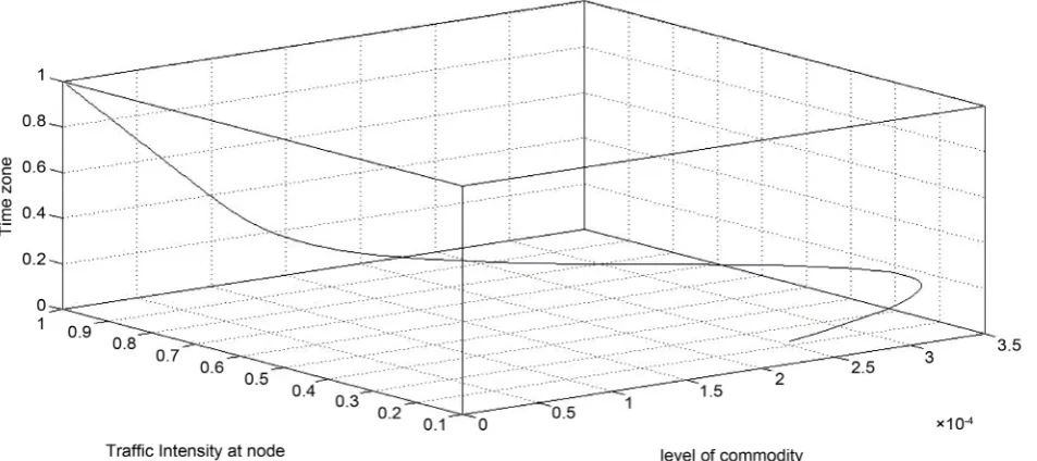
The Figure A2 illustrates about the effect of traffic intensity of commodity. Initially, when it increases then corresponding level of commodity also increases but after some time duration it may be cause of decrease of level of commodity at the node.
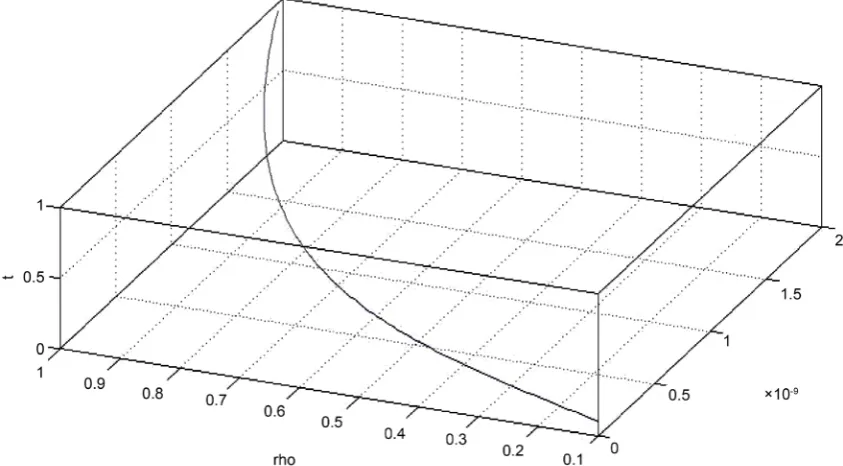
In the Figure A3, when the size parameter remains constant then we observe that with the increase in the traffic intensity of the commodity, the level of commodity also increases. It is seen that traffic intensity increases till certain level and after that it starts decreasing but level of commodity does not decrease, it gradually increases.
From Figure A4, it is clear that at a particular time when the node has con-stant value of stress parameter then the level of commodity previously increases with increase in the size parameter but after certain limit it begins decreasing in the level of commodity with increase in the size parameter.
5.2. Case-II
5.2.1. Observations from the Tables
From Table A7(a), it shows that if β lies from 1 to 1.25 and traffic intensity remains constant then the level of commodity becomes zero. After this range, increase in the amount of flow is reported but stress parameter remains constant then the level of commodity decreases.
From Table A8(b) and Table A9 we conclude that if we increase in the traffic intensity for the size parameter lies between 1 and 1.5, then the level of com-modity increases. But if we increase in the amount of flow then it has decreasing pattern of level of commodity.
From the Table A9, Table A10(a) and Table A10(b), we observe that the op-timal inflow quantity increases if 1) the traffic intensity as well as size parameter, stress parameter increases; 2) the value of size parameter and the stress parame-ter decrease as well as the amount of flow and traffic intensity increase; 3) the amount of flow increases but the optimal inflow quantity decreases when the amount of flow, size parameter and stress parameter increase.
5.2.2. Observations from Figures
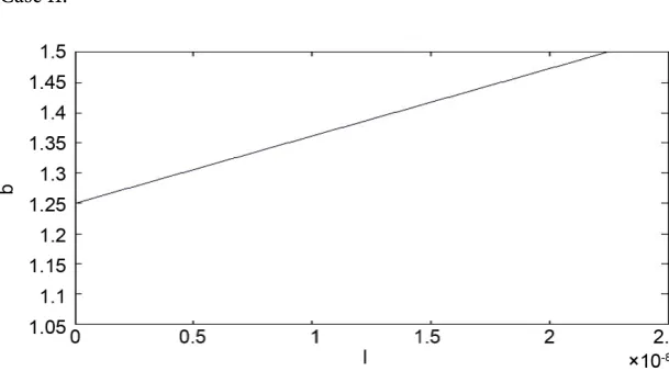
is no change in the level of commodity but when size parameter increases from 1.25 to 1.5, the level of commodity also increases.
Figure A6 shows that change in the amount of flow from 0 to 1.25, there oc-curs no change in the level of commodity. But from change in amount of flow 1.25 to 1.3, a very small change in the level of commodity takes place and after change 1.3 to 1.4, in the amount of flow the level of commodity also linearly in-creases but change in the amount of flow from 1.4 to 1.5 the level of commodity very rapidly increases. We may conclude from the observation that the level of commodity increases linearly with amount of flow. Moreover, if certain amount of flow linearity increases then this level of commodity increases rapidly.
6. Conclusion
Upon deeply analyzing the node wise level of commodity in the supply chain and total minimum variance cost of the network, we have been able to draw close observations under the sensitivity analysis of the model. By which we con-clude that this model is very sensitive about the size parameter of the system which proves the rationale of the value of the flow at any node as an important performance measure of the system. On the basis of level of commodity, we have computed the economic inflow quantities (optimal inflow quantity), and ob-tained the total minimum variance cost of the network under the subject to the conditions with non-negative constraints. These results have a vast spectrum of application in various fields of network such as network of communication, supply chain network and commodity (gas, oil and energy etc.) flow network. In order to control the flow of commodity (overflow on buffer stock), this model is very useful. This model paves the path to measure the level of commodity during flow in the random network. To measure and quantify the level of commodity at any node under uncertain environment of flow of commodity and to find the effect of the price on the flow of commodity would be our future research.
References
[1] Ahuja, R.K., Goldberg, A.V. Orlin, J.B. and Tarjan, R.E. (1992) Finding Mini-mum-Cost Flows by Double Scaling, Mathematical Programming, 53, 243-266.
https://doi.org/10.1007/BF01585705
[2] Ahuja, R.K., Magnanti, T.L. and Orlin, J.B. (1993) Network Flows: Theory, Algo-rithms and Applications. Prentice Hall, Englewood Cliffss, NJ.
[3] Bertsekas, D. and Gallager, R. (1992) Data Networks. 2nd Edition, Prentice Hall, Englewood Cliffs, New Jersey.
[4] Mishra, S.S. and Mishra, P.P. (2012) Phase Wise Supply Chain Model of EOQ with Normal Life Time for Queued Customers: A Computational Approach. American Journal of Operation Research, 2, 296-307.https://doi.org/10.4236/ajor.2012.23036 [5] Mishra, S.S. and Singh, P.K. (2011) Computational Approach to an Economic
Or-der Quantity Model with Power form Stock Dependent Demand and Cubic Deteri-oration. American Journal of Operation Research, 1, 5-13.
Mathematics with Applications, 61, 921-932.
https://doi.org/10.1016/j.camwa.2010.12.040
[7] Mishra, S.S., Yadav, S.K. and Rawat, S. (2015) Inventory Flow in Supply Chain with Deteriorating Items for Customer in Queue: Computation of Profit Optimization in Fuzzy Environment. American Journal of Operations Research, 5, 1-8.
[8] Jose, L., Yu, M. and Rexford, J. (2011) Online Measurement of Large Traffic Aggre-gates on Commodity Switches. Princeton University, Princeton.
[9] Gill, P., et al. (2008) Network Information Flow in Network of Queues. IEEE Inter-national Symposium on Modeling, Analysis and Simulation of Computers and Tel-ecommunication Systems, MASCOTS 2008, Baltimore, 8-10 September 2008, 1-8. [10] Thomas, C., et al. (2012) A Passive Measurement System for Network Test Beds.
Book on Lecture Notes of the Institute for Computer Sciences, Social Informatics a Telecommunications Engineering, 44, 130-145.
https://doi.org/10.1007/978-3-642-35576-9_14
[11] Narasimhan, T.N. (1999) Fourier’s Heat Conduction Equation: History, Influence, and Connections. Reviews of Geophysics, 37, 151-172.
https://doi.org/10.1029/1998RG900006
[12] Farlow, S.J. (1993) Partial Differential Equations for Scientists and Engineers. Dov-er, Mineola.
[13] Sifaleras, A. (2013) Minimum Cost Network Flows: Problems, Algorithms and Software. Yugoslav Journal of Operation Research, 23, 3-17.
https://doi.org/10.2298/YJOR121120001S
[14] Fonoberova, M. and Rebennack, F.S. (2010) Alogorithms for Finding Optimal Flows in Dynamic Networks. In: Rebennack, S., Pardalos, P.M., Pereira, M.V.F. and Iliadis, N.A., Eds., Handbook of Power System II, Springer, Berlin, 31-54.
https://doi.org/10.1007/978-3-642-12686-4_2
[15] Fonoberova, M. and Lozovanu, D.D. (2005) The Minimum Cost Multicommodity Flow Problem in Dynamic Networks and an Algorithm for Its Solving. Computer Science Journal of Moldova, 13, 29-36.
[16] Sisman, B. (2012) Supply Chain Network Design Considering Customer Service Level. Proceeding of the International Conference on Industrial Engineering and Operations Management, Istanbul, 3-6 July 2012, 2250-2258.
[17] Shah, R. and Ward, P.T. (2009) Defining and Developing Measures of Lean Produc-tion. The TQM Journal, 21, 127-142.
[18] Mishra, S.S., Mishra, P.P. and Sharma, S.K. (2012) Trait Analysis of Investment Packages as Using Computational Technique: A Case Study of Insurance Compa-nies. ESMSJ, 2, 22-28.
[19] Mishra, S.S. and Mishra, P.P. (2008) Price Determination for an Economic Order Quantity (EOQ) Model for Deteriorating Items under Perfect Competition. Inter-national Journal of Computer and Mathematics with Application, 56, 1082-1101.
Appendix 1
Table A1.
(
Ix t,verses , , ,β α ρ ξ)
.β α ρ ξ Ix t,
0.100 100 0.1 100 0.3704
0.100 200 0.1 100 0.0133
0.300 100 0.1 100 0.0319
0.300 100 0.1 400 0.0044
[image:13.595.207.540.266.377.2]0.300 100 0.1 500 0.0032
Table A2.
(
Ix t,verses , , , and β x t ξ)
.β x t ξ Ix t,
0.1 100 100 100 0.0620
0.1 200 100 100 0.1338
0.1 300 100 100 0.2100
0.4 400 400 400 0.0008
[image:13.595.206.538.417.489.2]0.5 500 500 500 0.0000
Table A3.
(
*)
verses , , , , and
q β α ρ x t ξ Ch = 50 cost unit, Co = 100 cost unit).
β α ρ x t ξ *
q
0.1 100 0.7 10 10 500 325.9247
0.2 100 0.7 15 20 500 248.4395
[image:13.595.210.540.528.622.2]0.3 100 0.7 20 30 500 175.8259
Table A4.
(
*)
verses , , , , and
q β α ρ x t ξ .
β α ρ x t ξ *( 07)
in e
q +
0.8 100 0.7 25 40 500 0.1312
0.8 100 0.7 30 50 500 0.2489
0.8 100 0.7 35 60 500 0.4286
[image:13.595.203.540.657.731.2]0.8 100 0.7 40 70 500 0.6875
Table A5.
(
*)
verses , , , , and
q β α ρ x t ξ .
β α ρ x t ξ *( 07)
in e
q +
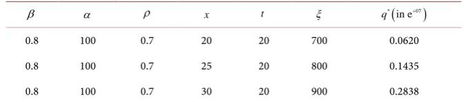
0.8 100 0.7 20 20 700 0.0620
0.8 100 0.7 25 20 800 0.1435
Table A6. (a)-(c)
(
*)
verses , , , , andq β α ρ x t ξ .
(a)
β α ρ x t ξ *( 08)
in e
q +
0.8 100 0.7 50 20 500 2.7703
0.8 100 0.7 50 20 600 2.5755
0.8 100 0.7 50 20 700 2.4215
0.8 100 0.7 50 20 800 2.2955
0.8 100 0.7 50 20 900 2.1899
(b)
β α ρ x t ξ *( 08)
in e
q +
0.8 300 0.7 50 20 700 0.7264
0.8 400 0.7 50 20 800 0.9182
0.8 500 0.7 50 20 900 1.0949
(c)
β α ρ x t ξ *( 08)
in e
q +
0.8 900 0.1 50 20 500 1.1448
0.8 900 0.2 50 20 600 1.4043
0.8 900 0.3 50 20 700 1.5529
Table A7.
(
Ix t,verses , , , and β x tξ α=100)
.β x t ξ ( 7)
, in e x t
I −
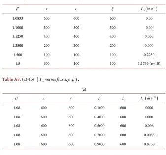
1.0833 600 600 600 0.00
1.1000 500 500 500 0.00
1.1250 400 400 400 0.000
1.2500 200 200 200 0.000
1.500 100 100 100 0.2250
1.5 600 100 100 1.1736 (e−10)
Table A8. (a)-(b)
(
Ix t,verses , , , ,β x t ρ ξ)
.(a)
β x t ρ ξ ( 66)
, in e x t
I −
1.08 600 600 0.1000 600 0000
1.08 600 600 0.4000 600 0000
1.08 600 600 0.5000 600 0.006
1.08 600 600 0.7000 600 0.0055
[image:14.595.202.540.434.749.2](b)
β x t ρ ξ Ix t,
1.500 100 100 0.1 600 0.2250 (e−7)
1.500 600 100 0.1 600 1.1736 (e−10)
1.5 100 600 0.7 600 0.1102 (e−5)
1.5 150 600 0.7 600 0.0218 (e−5)
1.5 200 600 0.7 600 0.0069 (e−5)
1.5 250 600 0.7 600 0.0028 (e−5)
Table A9.
(
*)
verses , , , , ,
q β α ρ x tξ .
β α ρ x t ξ *( 08)
in e
q +
1.1 900 0.1 50 20 500 1.1448
1.2 900 0.2 50 20 600 1.4043
[image:15.595.205.541.334.460.2]1.3 900 0.3 50 20 700 1.5529
Table A10. (a)
(
*)
verses , , , , ,
q β α ρ x tξ . (b)
(
*)
verses , , , , ,
q β α ρ x tξ .
β α ρ x t ξ *( 09)
in e
q +
1.4 900 0.8 80 20 800 0.2095
1.5 900 0.8 90 20 900 0.2178
1.5 900 0.8 100 20 700 0.2629
1.5 900 0.8 110 20 700 0.3607
1.5 900 0.8 120 20 700 0.4801
1.5 900 0.8 130 20 700 0.6233
1.5 900 0.8 140 20 700 0.7924
[image:15.595.62.539.504.716.2]Case I:
Figure A2. Rho (traffic intensity), time and level of commodity when size parameter β varies.
Figure A3. Traffic intensity (rho), level of commodity and time when size parameter β is constant.
[image:16.595.115.539.571.717.2]Case II:
Figure A5. Level of commodity and size parameter (beta = b).
Figure A6. Amount of flow and level of commodity.
Appendix 2
Some proofs are given below
Case II When β ≠1 and Let Constant
t
θ ∂
∅ = =
∂
2 2
, ,
1 2
,
x t x t
x t
I C I
t Iβ− x
∂ ∂
=
∂ ∂ ,
{ }
(
)
(
)
(
)
( )
1 1 2
2 1
, 2 2 2
2 1 1
1
x t
I C x C t
β
β β ξ β
αβρ β
−
−
+
= −
−
(
)
(
)
1 1
2
1 1
,
2 1 1
x t
x I
t
β β
ξ β
αβρ β
− −
+
= −
Since,
(
(
)
)
1 1
2
1 1
,
2 1 1
x t
x I
t
β β
ξ β
αβρ β
− −
+
= −
, so demand rate can be expressed as below.
(
)
(
)
2
1 1
, 2 1
1
x t
D x
t t
β β
β β
ξ β
α
αβρ β
− −
∂ +
=
It implies that
(
)
(
)
2 1 2 2 1 1 1 1 , 2 1 1 x t x
D x t C
t β β β β β β β β ξ β α αβρ β − − − − − + = ⋅ + − ⇒
Let the initial condition be D0,0 =0 then C=0,
Hence,
(
(
)
)
(
(
)
)
2 1 2 1
1 1
,
2 1 1 1 1 2
x t
D x t
β
β β
β
β β
ξ β β
α
αβρ β β
− − − − + − = − − ⋅ 2 2 , , 1 2 ,
x t x t
x t
I C I
t Iβ− x
∂ ∂
=
∂ ∂ , let Ix t, =X x T t
( ) ( )
⋅ be a solution and use the method of separation of variables to solve the partial differential equation. We get2 2 2 2 d d d d T X
X C T
t x
β = −β and 2
2 2 2
1 d 1 d
d d
T X
l t
C T −β = Xβ x = which in turn gives
us
(
)
(
2)
11 11
T = β− C lt+c β−
2 2 1 d d X l
Xβ x =
If
(
)
(
)
( )
2 2 2 1 1l β C
β + =
− then
{
}
2 1 1 2
X C C x β
−
= + is a solution to differential
equation. Further,
(
)
(
2)
11 3 2 2 1 d 1 d Tl T C lt C
t C T
β
β β −
− = ⇒ = − +
{
}
2(
)
(
)
12 1
1
, 1 2 1 3
x t
I C C x β β C lt C β
− −
= + − +
{ }
2(
)
(
)
12 1
1
0,t 1 1 3 0 1 0
I C β β C lt C β C
− −
= − + = ⇒ =
{ }
2(
)( )
11 1
,0 2 1 3 0 3 0
x
I C x β β C β C
− − = − = ⇒ =
{ }
(
)
(
)
(
)
( )
1 1 2 2 1, 2 2 2
2 1 1
1
x t
I C x C t
β
β β ξ β
αβρ β − − + = − −
(
)
(
)
1 1 2 1 1 , 2 1 1 x t x I t β β ξ β αβρ β − − + = − Since
(
(
)
)
1 1 2 1 1 , 2 1 1 x t x I t β β ξ β αβρ β − − + = −
so demand rate can be expressed as below.
(
)
(
)
2
1 1
, 2 1
(
)
(
)
2 1 2 2
1 1
1 1
,
2 1 1
x t
x
D x t C
t
β β
β β
β β
β β
ξ β
α
αβρ β
−
− −
− −
+
= − ⋅ +
Let the initial condition be D0,0 =0 then C = 0,
(
)
(
)
2 1 2 2
1 1
1 1
,
2 1 1
x t
x
D x t
t
β β
β β
β β
β β
ξ β
α
αβρ β
−
− −
− −
+
= − ⋅
When β ≠0 then there are following two cases arise as
Case-IIB
(
If β >1)
, If β >1 then(
)
(
)
( )
(
(
)
)
( )
22 log
1 1 1 2
2
1 1 1 1 1 1
1
, ,
1 1 1
1 e
2 1 2 1
it
x t x t
x
I I
t x
β β β β β
β
β αβρ β αβρ
β ξ β ξ
− − − − −
−
− −
= + − ⇒ = +
Submit or recommend next manuscript to SCIRP and we will provide best service for you:
Accepting pre-submission inquiries through Email, Facebook, LinkedIn, Twitter, etc. A wide selection of journals (inclusive of 9 subjects, more than 200 journals)
Providing 24-hour high-quality service User-friendly online submission system Fair and swift peer-review system
Efficient typesetting and proofreading procedure
Display of the result of downloads and visits, as well as the number of cited articles Maximum dissemination of your research work