Gauss Legendre Iterative Methods and Their Applications on Nonlinear Systems and BVP ODEs

(1)

http://www.scirp.org/journal/jamp ISSN Online: 2327-4379

ISSN Print: 2327-4352

Gauss-Legendre Iterative Methods and Their

Applications on Nonlinear Systems and BVP-ODEs

Zhongli Liu1*, Guoqing Sun2

1_{College of Biochemical Engineering, Beijing Union University, Beijing, China} 2_{College of Renai, Tianjin University, Tianjin, China}

Abstract

In this paper, a group of Gauss-Legendre iterative methods with cubic convergence for solving nonlinear systems are proposed. We construct the iterative schemes based on Gauss-Legendre quadrature formula. The cubic convergence and error equation are proved theoretically, and demonstrated numerically. Several numerical examples for solving the system of nonlinear equations and boundary-value problems of non-linear ordinary differential equations (ODEs) are provided to illustrate the efficiency and performance of the suggested iterative methods.

Keywords

Iterative Method, Gauss-Legendre Quadrature Formula, Nonlinear Systems, Third-Order Convergence, Nonlinear ODEs

1. Introduction

We consider the general form of a system of nonlinear equations as follows:

( )

(

( ) ( )

( )

)

T 1 , 2 , , n 0

F x = f x f x  f x = , (1)

where F D: ⊆Rn →Rn is a given nonlinear vector function, and each function

( )

i

f x can be thought of as mapping of a vector x=

(

x x₁, ₂,,xn

)

T, which is the n-

dimensional space n

R into the real number R.

Numerical solutions for systems of nonlinear equations have always appealed greatly to people in scientific computation and engineering fields. Some boundary-value prob-lems of nonlinear ordinary differential equations (ODEs) can be transformed to nonli-near systems like (1) by the finite difference method. Constructing an efficiently itera-tive method to approximate the root ξ∈D (such that F

( )

ξ =0) of Equation (1) is a How to cite this paper: Liu, Z.L. and Sun,

G.Q. (2016) Gauss-Legendre Iterative Me-thods and Their Applications on Nonlinear Systems and BVP-ODEs. Journal of Applied Mathematics and Physics, 4, 2038-2046.

http://dx.doi.org/10.4236/jamp.2016.411203

Received: October 24, 2016 Accepted: November 15, 2016 Published: November 18, 2016

http://creativecommons.org/licenses/by/4.0/

(2)

typical and important issue in nonlinear numerical computation. The Newton’s me-thod (see [1][2]) is one of the widely used methods for solving nonlinear equations by iteration as follows:

( )

1

( )

1 , 0,1, 2,

k k k k

x+ =x −F x′ − F x k= , (2) where

( )

1

F x′ − is the inverse of first Fréchet derivative F x′

( )

which is a Jacobian matrix of the nonlinear vector function F x

( )

. It converges quadratically when an ini-tial guess value x0 is close to the root ξ of Equation (1). In recent years, several iterative methods have been used to solve nonlinear equations and systems of nonlinear equations. In order to improve the order of convergence, a few two-step variants of Newton’s methods with cubic convergence have been proposed in some literature [3]-[11] and references therein for solving systems of nonlinear equations. S. We era- koon and T. Fernando [5] using the Newton theorem

( )

d

n

x n x

f x = f x +

∫

f′ t t,

proposed the Newton-type method with third-order convergence for nonlinear equa-tion and systems. M. Darvishi and A. Barati [6] received a third-order convergence iterative method based on Adomian decomposition method to the systems of nonlinear equations. M. Frontini and E. Sormani [7] presented third-order midpoint-methods using numerical quadrature formula. A. Cordero and J. R. Torregrsa [8] developed third-order convergence Newton-Simpson’s method and Open Newton’s method using the simple Simpson’s rule and an open quadrature formula of high order respectively. These are all classic two-step Newton-type methods to approximate the root of a system of nonlinear equations.

In Section 2 of this paper, we propose a group of two-step iterative methods with third-order convergence by Gauss-Legendre quadrature formula [12]:

( )

1

d

2 2 2

n b

i i

a

i

b a a b b a

f x x w f t

=

−  + − 

= _ + _

 

∑

∫

, (3)

where the necessary symmetrical conditions is 2

i

w =

∑

,

∑

ti=0,

∑

w ti i=0. (4)

Several numerical examples are provided in Section 3 using Gauss-Legendre iterative method for solving systems of nonlinear equations and boundary-value problems of nonlinear ODEs, and we finally make conclusions in Section 4.

2. The Iterative Methods and Cubic Convergence

Assume : n n

F D⊂R →R be a Fréchet differentiable function in a convex n D⊂R .

We have the mean-value theorem of multivariable vectors function F(x) in [1]:

( )

1

(

)

(

)

0 d ,

k k k k

F x −F x =

∫

F′ x +t x−x x−x t (5)

Using the left rectangular integral rule:

(

)

(

)

(

)

( )(

)

1

0F′ xk+t x−xk x−xk dt≈F′ xk x−xk ,

∫

(6)

(3)

Now, we apply the Gauss-Legendre quadrature formula (3) to approximate the integral on the right side of Equation (5), that is,

(

)

(

)

(

)

(

)

1 0

1 2

d 1 ,

2 2

n

k k

k k k i i k

i

x x x x

F x t x x x x t w F t x x

= + −   ′ + − − ≈ ′_ + _ −  

∑

∫

(7)

and using F x

( )

=0 we have

( )

1 1 2 2 2 n k k

k i i n

i

x x x x

x x w F t F x

−

=

 _′ + −  − ≈ − _ _ + __

 



∑

 . (8)

Herein, taking x as the next iterative step of xk, we get the following implicit

struc-ture:

( )

1 1 1 1 1 2 2 2 n

k k k k

k k i i n

i

x x x x

x x w F t F x

− + + + =  _′ + −  = − _ _ + __  



∑

 . (9)

We use the k-th iteration yk of the Newton’s method to replace xk+1 on the right side of the expression (9), and we construct the following group of two-step iterative schemes:

( )

1 1 1 1 2 2 2

k k k k

n

k k k k

k k i i k

i

y x F x F x

x y y x

x x w F t F x

− − + =  ₌ ₋ _′   _ _ ₊ ₋ __ ′ = − +  _ _ __      

∑

. (10)

We state and prove the convergence theorem for the schemes (10) as follows:

Theorem Let : n n

F D⊂R →R be a k-time Fréchet differentiable function in a convex set D with a root ξ ⊂D and x0 be close to ξ, then the group of iterative methods (10) is cubically convergent, and the error equation is

( )

2 2 3 4

1 2 3 3

1 3

2 8

n

k i i k k

i

e₊ C C w t C e O e

=

   

=_ − + _ + _ _ +

 



∑

 . (11)

Proof. As F

( )

ξ =0, and noting that x_k− =ξ e_k,

( )

_{( )}

1 ! k k F C F k ξ ξ − ′ = _.

By Taylor’s expansion, we have

( )

( )(

)

( )(

)

( )(

)

(

)

( )

2 3 4

2 4

2 3

1 1

2! 3!

,

k k k k k

k k k k

F x F x F x F x O x

F e C e C e O e

ξ ξ ξ ξ ξ ξ ξ

ξ

′ ′′ ′′′

= − + − + − + −

 

′

= _ + + _+ (12)

and

( )

2

( )

3

2 3

k k k k

F x′ =F′ ξ _I+ C e + C e +O e _. (13)

Then, suppose that

( )

1

( )

1

( )

1

k k

F x′ − = D e − _F′ ξ − , (14)

where

( )

2

( )

3

2 3

k k k k

D e = +I C e + C e +O e . (15)

(4)

( )

1 2

k k k

D e − = +I K e +K e ,

where K1 and K2 will be satisfied the definition of the following inversion.

( ) ( )

1

( )

1

( )

k k k k

D e D e − =D e − D e =I. (16) That is

(

2

)(

2

)

2 3 1 2

2 _n 3 _n _n _n

I+ C e + C e I+K e +K e =I. (17)

From (17), we have

2 1 2 2, 2 4 2 3 3

K = − C K = C − C . (18)

Therefore,

( )

1

(

2

)

2

( )

1

2 2 3

2 4 3

k k k

F x′ − =_I− C e + C − C e +_F′ ξ − . (19)

And

( )

(

)

(

)

(

)

( )

1 2 2 2 3

2 2 3 2 3

2 2 3 4

2 2 3

2 4 3

2 2 .

k k k k k k k

k k k k

F x F x I C e C C e e C e C e

e C e C C e O e

− _ _

′ =_ − + − + _× + + +

= − + − +

 

(20)

By the first step of (10), we have

(

)

( )

2 2 3 4

2 2 3 2

k k k k

y = +ξ C e + C −C e +O e = + ∆ξ , (21)

Here, suppose 2

(

2

)

3

( )

4

2 k 2 3 2 k k

C e C C e O e

∆ = + − + .

So,

1 1 1 1

2 2 2 2 2

k k

x y

x e

ξ ξ

+ _{= +} _{+ ∆ = +} _{+ ∆}

, (22)

(

)

1 1 1 1

2 2 2 2 2 2

k k

y x

e e

ξ _ξ

−

= + ∆ − + = − + ∆. (23) Furthermore,

(

)

(

)

1 1

2 2 2 2

k k k k

i i k i k

x y y x

t ξ t e t ξ d

+ −

+ = + − + + ∆ = + _{, (24)}

where,

(

)

(

)

1 1

2 2

k i k i

d = −t e + +t ∆. (25)

Then,

( )

(

)

( )

(

)

(

)

(

)

( )

(

)

(

)

(

)

( )

2

2 3

2 2 3

2

2 2 2 3

2 2 3

2 2

2 3

3

1 1 1

4 3

1 1 1 .

4

k k k k

i

k k

i k i i k k

i k i k i k k

x y y x

F t

F I C d C d

F I C t e C t C t e O e

F I C t e C t e C t e O e

ξ

+ −

 

′_ + _

 

′

= + + +

 

′

= _ + − + + ∆ + − + _

 

 

′

= _ + − + + + − + _

 



(26)

(5)

( )

(

)

(

)

(

)

( )

(

)

(

)

(

) ( )

1

2

2 2 2 3

2 2 3

1

2 2 2 2 3

2 2 3

1 1 1 1

2 2

3

1 1 1

4

3

1 1 1 2 .

4 n

k k k k

i i

i n

i i k i k i k k

i

n n n n

i k i i k i i k i i i k

i i i i

x y y x

w F t

w F I C t e C t e C t e O e

w I C e w t C e w t C e w t t O e

B F ξ ξ = = = = = = + −   ′_ + _     ′ _ + − + + + − + _    ₊ ₋ ₊ ₊ ₊ ₋ ₊ ₊  = =    =  ′

∑

(27)

By the conditions (4), we have

( )

2 2 2 2

( )

3

2 2 3

1 3

2 2 2 2

4

n

k k k i i k

i

B F ξ I C e C e C e w t O e

=  ₊ ₊ ₊  ₊ ₊    ′ _ = _  



∑

. (28)

So the iterative schemes (10) can be written as 1

( )

1 2

k k k

x₊ =x − B F x− . Subtracting

ξ from both sides of this equation, we can obtain

( )

1

1 1

2Bek+ =2Bek−F xk , (29)

that is

( )

(

)

( )

(

)

( )

2 2 2 3 3 2 4

2 1 2 2 3

1

2 3 2 3 4

2 3 3

1 3 2 8 3 2 8 n

k k k k k k k i i k k

i n

k i i k k

i

I C e O e e e C e C e C e w t O e F x

C C e C w t e O e

+ = =   + + = + + + _ + _+ −     = − + _ + _ +  

∑

(30)

Therefore, the error equation is

( )

2 2 3 4

1 2 3 3

1 3

2 8

n

k i i k k

i

e+ C C w t C e O e

=

   

=_ − + _ + _ _ +

 



∑

 . (31)

This shows that the group of iterative methods (10) is third-order convergent. As for the iterative methods (10), when n=1,w1=2,t1=0, then it can be trans-formed to the following form:

( )

1 1 1 2

k k k k

k k

k k k

y x F x F x

x y

x x F F x

− − +  = − ′   _ ₊ _ ′ = −  _ _   

. (32)

When n=2,w1=w2=1,t1=µ,t2= −µ, µ∈R is a parameter, then the methods (10) can be written as follows:

( )

1 1 1 1 2

2 2 2 2

k k k k

n

k k k k k k k k

k k k

i

y x F x F x

x y y x x y y x

x x F µ F µ F x

− − + =  ₌ ₋ _′   _ _ ₊ ₋ _ _ ₊ ₋ __ ′ ′ = − − + +  _ _ _ _ __        

∑

. (33)

Especially, we take the parameter µ=0.577350 in the iterative method (33) to

make applications in the following section.

3. Numerical Examples

The iterative method (33) with µ=0.577350 is demonstrated for solving systems of

(6)

Example 1. Consider a system of nonlinear equations with variables n=5:

(

)

2 1,

1 0, 1

n

j i

j j i

x n x i n

= ≠

− − = ≤ ≤

∑

, (34)

where x0 =

(

2, 2, 2, 2, 2

)

′ is the guess value. We can get the exact solution ξ =

(

1,1,1,1,1

)

′

by the iterative method (33) for Equation (34). The numerical results are shown in Ta-ble 1, in which k refers to the number of iterations.

Example 2. Consider solving the following two-point boundary-value problem of nonlinear ODE:

( )

0, 0,1

0 0, 1 1

x t x t t

x x

 ′′ + = ∈

 

= =

 (35)

We discretize the nonlinear ODE (35) with the finite difference method. Taking nodes ti =ih, where h=1N and N=10 herein, we can obtain the following

sys-tem of nine-variables nonlinear equations:

2

1 1 2

2

1 1

2

8 9 9

2 0

2 0, 2, 3, , 8

2 1 0

i i i i

x h x x

x x h x x i

x x h x

− +

 − − =

₋ ₊ ₋ ₋ ₌ ₌ 



− + − − = 

 , (36)

where x0=

(

1,1,1,1,1,1,1,1,1

)

′. Using the iterative method (33), we get the numerical

solutions ξ of Equation (36), that is,

(

)

0.1283710267934016 , 0.2531591633178528 , 0.3729158073866021 ,

0.4865657681707311 , 0.5932403023143547 , 0.6922126270196785 ,

0.7828650200725204 , 0.8646694471440053 , 0.9371751138295893 .

ξ =

′

  

The numerical results for the system of nonlinear Equations (36) derived from ODE (35) are shown in Table 2.

[image:6.595.193.556.561.617.2]

According to results of the above two numerical experiments, the iterative method (33) can achieve third-order convergence for systems of nonlinear equations, and their numerical solutions show also the method is feasible.

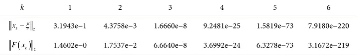
Table 1. The numerical solutions and errors of the system of Equation (34) using the method (33).

k 1 2 3 4 5 6

2 k

x −ξ 3.1943e−1 4.3758e−3 1.6660e−8 9.2481e−25 1.5819e−73 7.9180e−220

( )k 2

F x 1.4602e−0 1.7537e−2 6.6640e−8 3.6992e−24 6.3278e−73 3.1672e−219

Table 2. The numerical solutions and errors of the system of nonlinear Equation (36).

k 1 2 3 4

2 k

x −ξ 4.9234e−4 5.63305e−14 8.6475e−17 8.6475e−17

( )k 2

[image:6.595.194.553.649.706.2]

(7)

Example 3. Solving the following two-point nonlinear boundary-value problem of ODE with exact solution:

( )

(

)

2

1

1 1

0 1, 1

2 y

e

x y

y y e−

 ′′ = + ′ 



= = + 



. (37)

The exact solution for this problem of ODE (37) is

( )

1

(

)

2

x x

e

y x = − +e . We now

find the numerical solutions using the present method and compare them with the ex-act solution y x

( )

.

By the finite difference method, partitioning the interval

[ ]

0,1 :

0 0 1 2 n1 n

x = <x <x <<x− <x , yi+1 =yi +h h, =1 n.

Let y0=y

( )

0 =1,y1=

( )

x1 ,,yn−1= y x

( )

n−1 , and

( )

(

)

1 0.5

n n

y =y x = e− +e . And using the numerical differential formula for the second derivative 1 1

2

i i i

i

y y y

y

h

− − + +

′′ = , and the first derivative i1 i_,

(

_{1, 2,} _, ₁

)

i

y y

y i n

h

+ −

′ = =  − , we take n=10 herein, and

hence obtain the following system of nonlinear equations with nine variables:

(

)

2

1 2 1 1 0, 1, 2, , 9

i i i i i

y− − y +y+ −h h + y+ −y = i=  , (38)

where ( )0

(

)

T

0, 0, 0, 0, 0, 0, 0, 0, 0

y = is an initial value. We obtain the approximate

nu-merical solutions of this problem with the method (33) (iteration number k = 5):

(

)

*

1.00412287612219 ,1.01834640006185 ,1.04286614560037 ,

1.07798462092560 ,1.12411585747856 ,1.18179111195371 ,

1.25166573656183 ,1.33452729205395 ,1.43130499800870 . y =

′

  

Comparison of the numerical results of the boundary-value problem of ODE (37) and the exact solutions y x

( )

i are shown in Table 3, in which xi refers to the

nodes.

[image:7.595.196.553.551.704.2]

The error comparisons of the numerical solutions and exact solutions at different nodes xi for solving the problem of ODE (37) are shown in Figure 1.

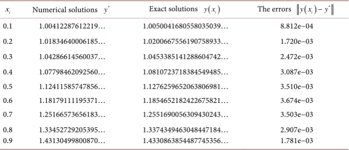
Table 3. Numerical comparison results for the problem of ODE (37).

i

x Numerical solutions *

y Exact solutions y x( )i The errors ( ) * i

y x −y

0.1 1.00412287612219… 1.0050041680558035039… 8.812e−04 0.2 1.01834640006185… 1.0200667556190758933… 1.720e−03 0.3 1.04286614560037… 1.0453385141288604742… 2.472e−03 0.4 1.07798462092560… 1.0810723718384549485… 3.087e−03 0.5 1.12411585747856… 1.1276259652063806981… 3.510e−03 0.6 1.18179111195371… 1.1854652182422675821… 3.674e−03 0.7 1.25166573656183… 1.2551690056309430243… 3.503e−03 0.8

(8)

[image:8.595.232.514.66.271.2]

Figure 1. Error comparisons for solving the problem of ODE (37).

4. Conclusion

In this paper, we construct a group of iterative methods with cubic convergence for the systems of nonlinear equations by using the Gauss-Legendre quadrature formula. Nu-merical results we gave are in consistence with the theoretical analysis, and meanwhile they also demonstrate that the presented scheme is efficient and feasible to solve sys-tems of nonlinear equations and to solve two-point boundary-value problems of nonli-near ordinary differential equations.

Acknowledgements

The work is supported by the Science and Technology Program of Beijing Municipal Commission of Education (No. KM201511417012).

References

[1] Ortega, J.M. and Rheinboldt, W.G. (1970) Iterative Solution of Nonlinear Equations in Several Variables. Academic Press, New York.

[2] Traub, J.F. (1964) Iterative Methods for the Solution of Equations. Prentice-Hall, Engle-wood Cliffs.

[3] Noor, M.A. and Noor, K.I. (2006) Improved Iterative Methods for Solving Nonlinear Equa-tions. Applied Mathematics and Computation, 183, 774-779.

https:/doi.org/10.1016/j.amc.2006.05.084

[4] Chun, C. (2006) A New Ityerative Method for Solving Nonlinear Equations. Applied Ma-thematics and Computation, 178, 415-422. https:/doi.org/10.1016/j.amc.2005.11.055

[5] Weerakoon, S. and Fernando, T.G.I. (2000) A Variant of Newton’s Method with Accele-rated Third-Order Convergence. Applied Mathematics Letters, 13, 87-93.

https:/doi.org/10.1016/S0893-9659(00)00100-2

[6] Darvishi, M.T. and Barati, A. (2007) A Third-Order Newton-type Method to Solve Systems of Nonlinear Equations. Applied Mathematics and Computation, 187, 630-635.

(9)

[7] Frontini, M. and Sormani, E. (2004) Third-Order Methods from Quadrature Formulae for Solving Systems of Nonlinear Equations.Applied Mathematics and Computation, 149, 771- 782. https:/doi.org/10.1016/S0096-3003(03)00178-4

[8] Cordero, A. and Torregrosa, J.R. (2007) Variants of Newtons Method Using Fifth-Order Quadrature Formulas. Applied Mathematics and Computation, 190, 686-698.

https:/doi.org/10.1016/j.amc.2007.01.062

[9] Noor, M.A. and Wasteem, M. (2009) Some Iterative Methods for Solving a System of Non-linear Equations. Computers and Mathematics with Applications, 57, 101-106.

https:/doi.org/10.1016/j.camwa.2008.10.067

[10] Hafiz, M.A. and Bahgat, M.S.M. (2012) An Efficient Two-Step Iterative Method for Solving System of Nonlinear Equations. Journal of Mathematics Research, 4, 28-34.

[11] Khirallah, M.Q. and Hafiz, M.A. (2012) Novel Three Order Methods for Solving a System of Nonlinear Equations. Bulletin of Mathematical Sciences & Applications, 1, 1-14.

https:/doi.org/10.18052/www.scipress.com/BMSA.2.1

[12] Guan, Z. and Lu, J.F. (1998) Numerical Analysis. High Education Press, Beijing.

Submit or recommend next manuscript to SCIRP and we will provide best service for you:

Accepting pre-submission inquiries through Email, Facebook, LinkedIn, Twitter, etc. A wide selection of journals (inclusive of 9 subjects, more than 200 journals)

Providing 24-hour high-quality service User-friendly online submission system Fair and swift peer-review system

Efficient typesetting and proofreading procedure

Display of the result of downloads and visits, as well as the number of cited articles Maximum dissemination of your research work