Explaining the durable goods co movement puzzle with non separable preferences: a bayesian approach

Munich Personal RePEc Archive

Explaining the durable goods

co-movement puzzle with non-separable

preferences: a bayesian approach.

Dey, Jaya and Tsai, Yi-Chan

Saint Louis University, National Taiwan University

20 December 2012

Online at

https://mpra.ub.uni-muenchen.de/57805/

Explaining the Durable Goods Co-movement Puzzle

with Non-Separable Preferences: A Bayesian Approach

∗

Jaya Dey

Saint Louis University

Yi-Chan Tsai

National Taiwan University

December 20, 2012

Abstract

A standard two-sector sticky price model with flexibly priced durables depicts nega-tive co-movement between durables and non-durables after a monetary policy shock, which is at odds with the empirical evidence. This paper proposes a new channel, non-separable preferences with a small wealth effect on labor hours, as a solution to the co-movement puzzle. In contrast to the standard model where the aggregate hours re-main relatively unchanged after the contractionary policy shock, aggregate labor hours fall along with the fall in the labor wage, thereby discouraging production in both the durable and non-durable goods sectors. We further compare our model’s explanatory power with two other alternatives that can resolve the puzzle by using a Bayesian approach. Based on the log marginal likelihood and cross-correlation function com-parison exercises, we find evidence that the data strongly favor both the alternative specifications over our baseline model. More specifically, the model with a working capital channel and habit formation gives the best fit to the data, especially for cross-correlations between durable and non-durable consumption.

Keywords: preferences; wealth effect; monetary policy; inflation; output

JEL classification: E21, E31, E32, E52

∗_{We thank Bill Dupor, Masao Ogaki, Jang-Ting Guo, Jeffrey Campbell, Hidehiko Ichimura, Takashi}

Kano, Ching-Sheng Mao and Hung-Ju Chen for useful comments and suggestions. We also thank session participants at 2012 Midwest Macroeconomics Meetings, 2011 SEA meeting, as well as seminar participants at Oklahoma State University, National Taiwan University and University of Tokyo. All errors are our own.

†_{Email: [email protected]}

1

Introduction

Erceg and Levin (2006), using a VAR approach, documented that expenditures on both durable and non-durable goods decrease after a contractionary policy shock. Standard New Keynesian models with different price setting behaviors in the durable and non-durable goods sectors have failed to replicate this result. In particular, with a flexibly-priced durable goods sector, a contractionary monetary policy shock leads to a decrease in non-durables but an increase in durable goods production, leaving the aggregate production unchanged. This

co-movement puzzle is first pointed out by Barsky, House and Kimball (2003, 2007, BHK hereafter).

We propose a new mechanism, namely, non-separable (in consumption and leisure) pref-erences with a small wealth effect on labor hours as a possible solution to the puzzle. By incorporating these preferences in the standard BHK setting, we find that outputs across sectors are able to comove after a monetary policy shock. Furthermore, by introducing in-ternal habit formation in non-durable consumption, we can generate high interest-elasticity in durable output relative to non-durable output as in the data. Next, we estimate our model using Bayesian techniques and the estimated model’s predictions are consistent with our intuition. Finally, using log marginal likelihood, we compare our model’s fit with two competing alternative model specifications in the literature that can resolve the puzzle in isolation. The out-of-sample forecasts indicate that the data strongly support both the al-ternatives over our model.

The preferences adopted here is first proposed by Greenwood, Hercowitz and Huffman (1998, GHH hereafter), who induce a zero wealth effect on labor supply. In the past two decades, these preferences have been widely employed in resolving famous puzzles based on US and international data. For example, GHH demonstrated that these preferences act as a possible channel to induce positive co-movement between output, consumption, and invest-ment after an investinvest-ment-specific technology shock, which standard preferences have failed to do. Raffo (2007, 2009) identify the potential for these preferences in explaining many key features of international business cycles. Monacelli and Perotti (2008) show that these preferences can bring about a rise in consumption and the real wage after a positive gov-ernment spending shock that is consistent with their VAR estimates. Recently, Jaimovich and Rebelo (2009) have introduced generalized GHH preferences that can generate positive co-movement amongst major macroeconomic aggregates after a positive news shock to fu-ture productivity. In this paper, we investigate the role of augmented GHH preferences in reconciling a standard two-sector model’s prediction with the empirical VAR counterparts.

which can resolve the co-movement puzzle.1 _{In particular, we compare our benchmark model}

with GHH preferences with two existing models given by Carlstrom and Fuerst (2006) and Tsai (2010). Carlstrom and Fuerst (2006) introduce nominal wage stickiness in the stan-dard model of BHK. Sticky wages induce price stickiness in durables, giving durable goods producers less incentive to adjust prices after a contractionary monetary policy shock. This leads to a decline in durable goods production along with non-durable goods production, resolving the co-movement puzzle. Tsai (2010) solves the puzzle by incorporating a work-ing capital channel and habit formation in non-durable consumption. After a contractionary monetary policy shock, production cost rises due to the working capital channel, leading to a fall in both durable and non-durable goods production. The consumption growth smoothing motive implied by habit formation further dampens the response of non-durable production after the shock. Similar to his paper, the mechanism suggested by our paper can solve the co-movement puzzle without directly or indirectly inducing price stickiness in the durable goods sector. Separately and more recently, Kim and Katayama (2011) also propose the non-separable preference as a possible solution for the co-movement problem. However, our approach is different from theirs in two ways. First, their specification of preferences is dif-ferent from ours and, secondly our paper provides systematic evaluation across models that can resolve the co-movement puzzle using a full information econometric strategy.

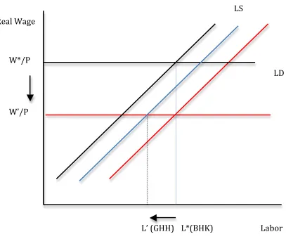
With separable preferences, due to the low depreciation rate of durables, the shadow value for durables remains relatively constant following transitory shocks, which induces aggregate labor hours and thus aggregate production to remain nearly constant. Thus, a decline in non-durable goods production after a contractionary monetary policy shock must be offset by an increase in durable goods production, giving rise to the co-movement puzzle. By contrast, aggregate hours fall along with the fall in the labor wage under non-separable GHH preferences, discouraging production in both the durable and non-durable goods sec-tors. This makes it possible for both durable and non-durable goods production to fall simultaneouly on impact, thereby resolving the co-movement puzzle.

This paper is also related to the growing literature on the estimation of general equi-librium models using Bayesian techniques that systematically evaluate the importance of various shocks and frictions in causing business cycle fluctuations.2 _{Using these techniques}

we find that our estimated model with intermediate habit persistence and the two

alterna-1

Other seminal work includes Kitamura and Takamura (2010) who address the issue by incorporating sticky information in the standard BHK setting; Levin and Yun (2011) who consider the role of incom-plete financial markets; and Sudo (2008) who presents an input-outut model, where non-durables act an intermediate inputs for durable production andvice-versa.

2

tive specifications can simultaneously make outputs in both sectors comove and induce high interest sensitivity in durables compared to non-durables after a monetary policy shock as in the data.

Finally, the Bayesian approach allows us to engage in a formal comparison between our model and two competing alternatives. Fern´andez-Villaverde and Rubio-Ram´ırez (2004) show that model comparisons, based on marginal likelihood, are consistent even when the models are misspecified. Rabanal and Rubio-Ram´ırez (2005) estimate and compare four versions of a sticky price New Keynesian model using Euro data. Another paper by Ichiue, Kurozumi and Sunakawa (2008) studies the role of an extensive margin in inflation dynamics by estimating and comparing three alternative models of labor adjustments. Following their approach, we compute each model’s marginal likelihood in order to compare their explana-tory power. We find that both of the competing alternatives outperform our benchmark model in fitting the data. In particular, the data strongly favor Tsai (2010) over all other specifications.

The rest of the paper is organized as follows. We present our model in Section 2 and the calibration results in Section 3. Section 4 presents the alternative models and Section 5 estimates the models. Section 6 discuss the results and compares the benchmark model with other alternatives, and Section 7 concludes.

2

Model

Our model is based on the framework developed in BHK (2007), Carlstrom and Fuerst (2006) and Tsai (2010). There are three types of agents in this economy: households, firms, and the monetary authority. We modify their models by incorporating GHH preferences. Households derive utility from the consumption of non-durable goods, durable goods and leisure. On the production side, there are two sectors: durable and non-durable goods sectors. In each sector, there is a continuum of monopolistically competitive intermediate firms, each producing a differentiated product. We describe their optimal behaviors as below.

2.1

Households

In every period, the representative household supplies labor (Lt), and chooses nondurable

consumption (Ct), a durable consumption stock (Dt), and a geometric average of current

and past consumption composite levels (Ht) to maximize expected lifetime utility

E0

∞

X

t=0

where β is the discount factor, and ǫg_t is the intertemporal preference shock that follows an AR(1) process:

ǫg_t =ρgǫg_t−₁+η g

t (2.1.1)

whereηg_t ∼N(0, σg) andU(Ct, Ct−1, Dt, Dt−1, Lt, Ht) is the augmented Jaimovich and Rebelo

(2009) utility function that takes the form

U(Ct, Ct−1, D_t, D_t−1, L_t, H_t) =

h

(ψc(Ct−hbCt−1)

ρ−1

ρ + (1₋ψ

c)ǫdt(Dt−hbDt−1)

ρ−1 ρ )

ρ ρ−1 ₋ǫl

tφL1+t νHt

i1−_σ

1−σ

where σ is the intertemporal elasticity of substitution, hb is the habit persistence, ψc is the

weight of nondurable goods in the household’s consumption composite, ρ is the elasticity of substitution between durable and nondurable consumption, ν is the inverse of the Frisch labor supply elasticity, andǫl

t is the intratemporal preference shock, also known as the labor

supply shock, which has the following law of motion:

ǫl_t=ρlǫl_t−₁+η l

t (2.1.2)

where ηl

t ∼N(0, σl). Also, ǫdt is the durable preference shock which has the following law of

motion:

ǫd_t =ρdǫd_t−₁+η d

t (2.1.2)

where ηd

t ∼ N(0, σd). The presence of Ht makes preferences time non-separable in a

con-sumption composite of durables and non-durables and hours worked. The law of motion for

Ht is

Ht =

h

(ψc(Ct−hbCt−₁)

ρ−1

ρ + (1₋ψ

c) (Dt−hbDt−₁)

ρ−1 ρ )

ρ ρ−1

i(γ) H1−_γ

t−₁ (2.1.3)

where γ ∈(0,1).

A representative household enters period t with initial bond holdings of St−₁, receives

wage income, WtLt, profits, Πt, and government transfers, Tt, and purchases non-durable

constraint is

Pc,tCt+Px,tXt+Px,t

1 2φ1

(Xt−δDt−₁)2

Dt−₁

≤WtNt+

X

j=c,x

Rj,tuj,tK¯j,t

+ Πt+Tt+St−₁−

St

Rt

− X

j=c,x

Pj,ta(uj,t) ¯Kj,t, t= 0,1, .. (1)

and the law of motion for durable goods consumption is

Dt= (1−δ)Dt−₁+X_t,

whereS−₁ and D−₁ are given and δis the depreciation rate. R_j,t,K_j,t and u_j,t are the rental

rate of capital, productive capital stock and variable capital utilization rate in each sector

j = c, x. Hence, the capital services in each sector is given by Kj,t = uj,tK¯j,t. The cost

of setting the capital utilization rate is given by a(uj,t) which is increasing and convex in

uj,t. We assume ¯uj = 1, a(1) = 0. Also, the parameter χ governs the elasticity of capital

utilization and is given by χ= a_a′′′₍₁₎(1).

By letting Bt =

h

ψc(Ct−hbCt−1)

ρ−1

ρ + (1₋ψ

c)ǫdt(Dt−hbDt−1)

ρ−1 ρ

i ρ ρ−1

and Vt = [Bt−

ǫl

tφL1+t νHt], the first-order conditions from the household optimization problem are:

Λt=ψcǫgtV −_σ t B 1 ρ t C −1 ρ

t +λtγB

ρ(γ−1)+1 ρ

t ψcC

−1 ρ

t H1 −_γ

t−₁ (2.1.5)

λt+ǫgtǫltV −_σ

t φL1+t ν =βEtλt+1(1−γ)Btγ+1H

−_γ

t (2.1.6)

ǫg_tǫl_tV−σ

t φ(1 +ν)LνtHt= Λt

Wt Pc,t (2.1.7) Λt Px,t Pc,t

=ǫg_tV−σ

t B

1 ρ

t ψdD

−1 ρ

t +λtγB

ρ(γ−1)+1 ρ

t ψdD

−1 ρ

t H

(1−_γ)

t−₁ +βEt(1−δ)Λt+1

Px,t+1 Pc,t+1

(2.1.8)

Λt

Pc,t

=βEt

Λt+1 Rt

Pc,t+1

Here λt and Λt represent the Lagrangian multipliers for constraints (2.1.3) and (2.1.4),

re-spectively. Equation (2.1.5) represents the marginal utility of non-durable consumption. Equations (2.1.7) represents the trade-off between non-durable consumption and leisure. Equation (2.1.8) represents the trade-off between non-durable and durable goods. Equation (2.1.9) represents the trade-off between non-durable consumption and bond holdings.

2.2

Firms

There are two types of firms: a continuum of non-durable goods producers and a continuum of durable goods producers. Non-durable goods firms set their prices `a la Calvo while durable goods firms can adjust their prices frictionlessly every period. These intermediate goods firms are competitive in the factor market, and take factor prices as given. I allow the factors to move freely within and between sectors.

2.2.1 Non-durable goods firms

There is a continuum of monopolistically competitive firms in the non-durable goods sector indexed by f ∈(0,1) that sell non-durable goods to final goods producers. They set a price

Pc,t(f) subject to a Calvo price setting. In each period, a fraction 1−θc of the firms in

this sector reoptimize their prices regardless of the time of their last price adjustment. The remaining fraction θc of the firms use the same price as in the previous period.

The demand faced by each firm depends on the price of its product and the total demand for non-durable goods

Ct(f) =

Pc,t(f)

Pc,t

−ε

Ct, (2.2.1.1)

whereCt =

hR1 0 Ct(f)

ε−1 ε df

i ε ε−1

is the consumption aggregator, andPc,t=

hR1

0 Pc,t(f) 1−ε

dfi

1 1−ε

represents the price index for non-durable goods. Production requires labor input

Ct(f) = (Kc,t(f))α(AtLc,t(f))1−α, (2.2.1.2)

where At denotes the aggregate productivity shock which has the following law of motion:

At=At−1e

ga,t _(2.2.1.3)

where ηa

t ∼N(0, σa).

A non-durable good producer f chooses P∗

c,t(f) so as to maximize its discounted profit,

max

P∗

c,t(f)

∞

X

j=0

(βθc)jEt

Λt+j

Pc,t+j

[Pc,t+j(f)Ct+j(f)−Wt+jLc,t+j(f)−Rc,t+jKc,t+j(f)]

subject to the demand for its product (2.2.1.1) and production function (2.2.1.2), where Λt+j

denotes the marginal utility of consumption for period t+j. The first-order conditions are,

Wt=M Cc,tKc,tα(1−α)(AtLc,t) −α

At (13)

Rc,t=M Cc,tK(α −₁₎

c,t (α)(AtLc,t)(1 −_α)

(14)

P∗

c,t(f) =

ε ε−1

P∞

j=0(βθc)

j

EtΛt+jM Cc,t+j

1

Pc,t+j

1−_ε

Ct+j

P∞

j=0(βθc)

j

EtΛt+j

1

Pc,t+j

1−_ε

Ct+j

, (15)

where M Cc,t is the marginal cost in the non-durable goods sector. The non-durable price

index is written as,

Pc,t=

(1−θc)P ∗₁−_ε

c,t +θcP1 −_ε c,t−₁

1

1−ε_{. (2.2.1.6)}

2.2.2 Durable goods firms

In the durable goods sector, there is a continuum of monopolistically competitive firms, and unlike the non-durable goods sector, durable goods firms reoptimize their prices every period, and face identical linear production and demand.

A durable goods firm f chooses its price P∗

x,t(f) so as to maximize its current profit,

max

P∗

x,t(f)

Px,t(f)Xt(f)−WtLx,t(f)−Rx,tKx,t(f),

subject to the production function

Xt(f) = Kx,tα (AtZtLx,t(f))1−α, (2.2.2.1)

and the demand function

Xt(f) =

Px,t(f)

Px,t

−_ε

where Xt =

hR1 0 Xt(f)

ε−1 ε df

i ε ε−1

, Px,t =

hR1

0 Px,t(f) 1−_ε

dfi

1 1−ε

, and Zt is the relative price

shock and follows:

Zt =Zt−1egz,t (2.2.2.3)

gz,t=ρzgz,t−₁+η_tz (2.2.2.4)

where ηz

t ∼N(0, σz). Note that, in equilibrium,

1

Zt

= Px,t

Pc,t

(2.2.2.5)

The first-order conditions are:

Wt=M Cx,tKx,tα (1−α)(AtZtLx,t) −_α

AtZt (19)

Rx,t =M Cx,tK(α −₁₎

x,t (α)(AtZtLx,t)(1−α) (20)

P∗ x,t(f) =

ε ε−1

Wt

AtZt

. (2.2.2.6)

where M Cx,t is the marginal cost in the durable goods sector.

2.3

Monetary policy and market clearing

The central bank follows the Taylor rule by adjusting the nominal interest rate in response to changes in inflation and the output gap.3 _{We allow the monetary authority to partially}

adjust toward the optimal interest target.

Rt=Rρt−r₁(πt)

(1−_ρr)φπ

(Yt)(1 −_ρr)φy

ǫr_t. (2.3.1)

whereρr determines the degree of interest rate smoothing andǫrt is an i.i.d. monetary policy

shock such that ǫr

t ∼N(0, σr).

2.4

Market Clearing

Finally, the model is closed with market clearing conditions in the labor and goods markets. The labor market equilibrium requires

Lt=Lc,t+Lx,t. (2.4.1)

3

Inflation is defined as a weighted average of nondurable goods inflation and durable goods inflation,

b

and the goods market equilibrium requires that

Yt =Ct+Xt. (2.4.2)

The de-trended model and the corresponding log-linear equations can be found in the appendix.

3

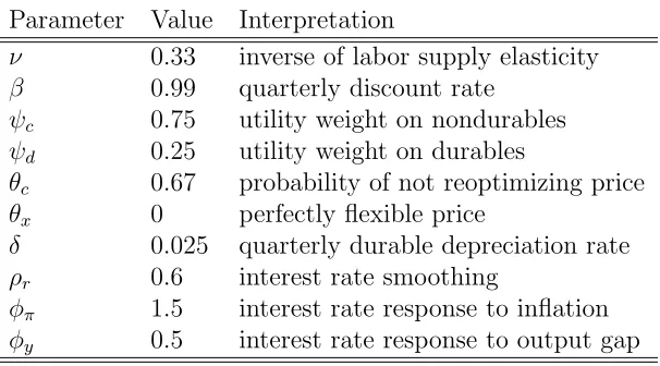
Table 1: Parameter values in the benchmark model Parameter Value Interpretation

ν 0.33 inverse of labor supply elasticity

β 0.99 quarterly discount rate

ψc 0.75 utility weight on nondurables

ψd 0.25 utility weight on durables

θc 0.67 probability of not reoptimizing price

θx 0 perfectly flexible price

δ 0.025 quarterly durable depreciation rate

ρr 0.6 interest rate smoothing

φπ 1.5 interest rate response to inflation

φy 0.5 interest rate response to output gap

Notes: The calibration value of the parameters in the benchmark model.

Most of the parameter values are taken from BHK (2007). We set the subjective discount factor, β, equal to 0.99, and the inverse of the Frisch labor-supply elasticity, ν, equals 0.33. The depreciation rate of durable goods,δ, is 0.025 which implies an annual depreciation rate of 10%. The intertemporal elasticity of substitution, σ, and the intratemporal elasticity of substitution between durables and non-durables, ρ, are both set equal to 1. The probability that a firm in the non-durable goods sector cannot reoptimize its price in any given period,

θc, is set to 2/3. We assume that the monetary authority partially adjusts its policy rate

toward the optimal interest target, and setρr = 0.6. Following the literature, we setφy = 0.5

and φπ = 1.5. The latter implies that the monetary policy rate responds more than

one-for-one to changes in inflation, and this ensures a unique equilibrium. Table 1 summarizes the parameter values.

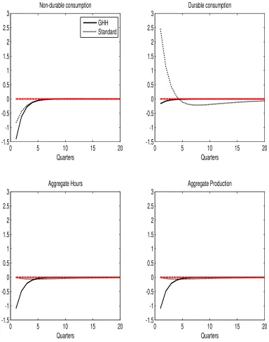
be-tween durables and non-durables as pointed out by BHK when the preferences are separable between the consumption composite and leisure. We then show that we can resolve the co-movement problem when we have non-separable preferences between the consumption composite and leisure which are the augmented GHH preferences. For these two cases, we setγ = 0 and γ = 1, respectively, and the results can be found in Figure 1.

To obtain the intuition of the mechanism between these two preferences, let us look at the case where γ = 1. When γ =σ =ρ= 1, Bt =Ht=CtψcDtψd and the period utility becomes

U(Ct, Dt, Lt, Ht) = logCtψcDψtd +log(1−ǫltφL1+t ν) which is the same class of preferences as

discussed in BHK. Equation (2.1.6) becomes λt =−ǫgtǫltV −₁

φL1+t ν. Equation (2.1.5) can be

simplified as Λt= ψ_Cc_t. Combining (2.1.5) and (2.1.7), we obtain the labor-leisure condition

φ(1 +ν)Lν t

1−φL1+ν =

Wt

Pc,t

ψcCt−1 =

ε−1

ε AtZt Px,t

Pc,t

ψcCt−1. (3.1)

The second equality follows by substituting out Wt using the price of durable goods, Px,t = ε

ε−₁ Wt

AtZt. Moreover, by plugging λt and Λt into equation (2.1.8), we obtain ψcC

−₁ t

Px,t

Pc,t =

ψdǫgtD1t +βψc(1−δ)EtC

−1 t+1

Px,t+1

Pc,t+1. With a small depreciation rate for durable goods, changes

in the stock of durable goods and its associated shadow value after a temporary policy shock are small, inducing only a small change in ψcCt−1

Px,t

Pc,t. Since the right-hand side of equation

(3.1) changes little in response to the monetary policy shock, aggregate labor hours remain relatively constant. Therefore any fall in non-durable production is associated with a rise in durable production, and the separable reference has difficulty generating co-movement between durables and nondurables.

Next, when γ = 0 and ρ = σ = 1, we obtain the augmented GHH preferences and the period utility becomes U(Ct, Dt, Lt, Ht) = log(CtψcD

ψd

t −ǫltφhLt1+ν) where Ht= Ht−₁ =

H = constant and φh = φH. If we revisit the leisure labor choice condition, equation

(2.1.7) now becomes φ(1 + ν)Lν

t = PWc,ttψc

Bt

Ct. Compared to the separable preferences, the

fall in non-durable goods consumption now induces a smaller wealth effect on labor supply as Dt remains relatively constant and the rise in B_Ct_t = (D_Ctt)1−ψc is smaller than the rise

in C−₁

t following the contractionary policy shocks.4’5 With a smaller wealth effect on the

labor supply decision, aggregate labor hours fall following a contractionary policy shock and

4

We refer to this as the augmented GHH labor-leisure condition. Unlike the typical GHH preference which only features non-durable goods consumption and induces labor supply depending only on the real wage, here labor supply depends on both the real wage and the fraction of the composite consumption to non-durable goods consumption. In the extreme case, where the composite consumption features only nondurable goods consumption (i.e.,ψc= 1), we get back the typical labor leisure choice under the standard

GHH preferences φ(1 +ν)Lνt = Wt

Pc,t. In that case, there is no wealth effect associated with labor supply

decisions.

5

therefore allow us to solve the co-movement problem between durables and non-durables. In response to a contractionary policy shock, we observe a fall in both non-durables and durables, and aggregate output falls. This is the resolution of the co-movement puzzle.

The JR preferences nest the KPR and GHH utility functions as special cases. From our discussion above, for a small value of γ, the JR preference is able to generate a fall in aggregate labor hours following a contractionary policy shock which enables our models to generate a fall in both the durable and non-durable goods sector and thus solves the co-movement puzzle.6

Fig. 2 shows the labor market equilibrium under both the separable preferences and the non-separable preferences. Under separable preferences, the wealth effect and the substitu-tion effects are roughly canceled out following the policy shocks, while under non-separable preferences, the substitution effects are larger than the wealth effect which leads to a fall in aggregate labor hours following a fall in the real wage in response to a contractionary policy shock.

Although our model can successfully resolve the co-movement puzzle, the fall in non-durables is larger than the fall in non-durables, which is inconsistent with the empirical finding that durables are more interest rate sensitive than nondurables. To reconcile this inconsis-tency between the model’s prediction and the empirical findings, we add in the habit forma-tion for non-durable consumpforma-tion. In particular,Bt= (Ct−hbCt−1)ψcDtψd and 0≤hb ≤1

which is the parameter governing habit persistence. The introduction of habit formation al-ters the propagation of policy shocks as the household dislikes large and rapid changes in non-durable goods consumption and therefore mitigates the initial fall in non-durables con-sumption which allows our model to generate a more interest rate sensitive durable goods response than non-durables and is consistent with the empirical findings.

4

Alternative Specifications

While several papers have used various channels in accounting for the co-movement puzzle, the existing literature lacks a formal comparison between competing alternatives using US data. We compare the explanatory power of our baseline model with augmented GHH preferences with two alternative channels in the literature. To this end, we extend the baseline BHK model in two different ways. First, following Carlstrom and Fuerst (2006), we introduce nominal wage rigidities and durable goods adjustment costs (Model 1). Second, in the spirit of Tsai (2010), we introduce a working capital channel in both durable and non-durable goods production and internal habit formation in non-non-durable goods consumption

6

(Model 2). Since the two extensions are well-known in the literature, here we only highlight the key equations in each model.

4.1

Model 1: Carlstrom and Fuerst (2006)

Carlstrom and Fuerst (2006) introduces nominal wage stickiness in the standard sticky price model of BHK to resolve the co-movement puzzle. Households have monopoly power over labor supply allowing for sticky nominal wages `a la Calvo (1983). Hence the wage is set according to the following equation:

ˆ

Wt=

β

1 +βWˆt+1+

1

1 +βWˆt−1 + β

1 +βπˆt+1+

(1−θwβ)(1−θw)

θw

h

ˆ

W_th−Wˆt

i

(4.1.1)

where (1−θw) denotes the fraction of households that adjust their wage at time t and ˆWth

is the marginal rate of substitution. Furthermore, to smooth the behavior of durable goods consumption, we add adjustment costs in the household budget constraint along the lines of Engel and Wang (2007):

Pc,tCt+Px,tXt+Px,t

1 2φ1

(Xt−δDt−₁)2

Dt−₁

≤WtNt+ Πt+Tt+St−₁−

St

Rt

, t = 0,1, .. (4.1.2)

whereφ1 is the adjustment cost parameter. The rest of the model is the same as benchmark setting. The details of the linearized model are given in the appendix.

4.2

Model 2: Tsai (2010)

A recent paper by Tsai (2010) explores the role of financial frictions as a possible solution to the co-movement puzzle. He extends the basic BHK model to include a working capital channel to both the durable and non-durable sectors which imposes a constraint on the firms to borrow in advance in order to pay wages. The log-linearized marginal cost becomes:

ˆ

M Ct= ˆWt+ ˆRt−Aˆt (4.2.1)

non-durable consumption becomes:

ˆ Λt=

1−σ

1−hβ h

ˆ

Bt−hβEtBˆt+1 i

− 1

(1−hβ)(1−h)

h

ˆ

Ct−hCˆt−₁

i

+ hβ

(1−bβ)(1−b)Et( ˆCt+1−bCˆt)+ 1 (1−βh) ǫ

g

t −βhEtǫgt+1

(4.2.2)

Again, please see the appendix for the rest of the linearized model.

5

Bayesian Estimation

In this section we describe the data, estimation methodology and the prior distributions of the parameters for all three model specifications.

5.1

Data and Methodology

Implementation of the Bayesian estimation requires several steps. The first step is writing the solution to the general equilibrium model in state-space representation:

xt+1 =h(xt) +ηǫt+1, (5.1.1)

yt =g(xt) +χut, (5.1.2)

where xt is a vector of state (both predetermined and endogenous) and control variables

and yt defines the vector of observables. ǫt and ut are the vectors of structural shocks and

measurement errors, respectively, and are distributed as N(0, I); and h(x), g(x), η, χ are functions of deep parameters of the model. The second step involves the formulation of the likelihood function of the solution system using the Kalman filter. The third step combines the likelihood function with the priors for the parameters to form the posterior density func-tion. Since the posterior distribution is nonlinear and a complicated function of the deep parameters, the final step involves computing it using sampling-like methods such as the Metropolis-Hastings algorithm.7

The sample period ranges from 1966:02 to 2003:01, at a quarterly frequency. Our ob-servables consist of five macro-economic time series: (i) real durable goods consumption,

7

(ii) real non-durable goods consumption, (iii) the relative price of non-durables to durables, (iv) hours worked, and (v) a short-term interest rate. The first three series are taken from the US Department of Commerce - Bureau of Economic Analysis databank. Both durable and non-durable goods consumption expenditures are deflated by their respective price de-flators to obtain real variables. The hours data series is taken from the Bureau of Labor Statistics (BLS). Hours (hours and hourly compensation for the NFB sector for all persons) are adjusted to take into account the limited coverage of the NFB sector compared to GDP (the index of average hours for the NFB sector is multiplied by the Civilian Employment (16 years and over). The short-term interest rate is the Federal Funds Rate. All series are seasonally adjusted. Our demeaned set of observable variables is given by:

Zt= [lNt, dlCt, dlDt, lRt, dlPt] ′

where l and dl stand for the log and log difference, respectively. Figure (3) plots the set of observables. The corresponding log-linearized measurement equations, mapping the observ-ables and transformed variobserv-ables, are as follows:

        lNt dlCt dlXt Rt dlPt         =         ˆ nt

(ˆct−ˆct−₁)

(ˆxt−xˆt−₁)

ˆ

rt

(ˆpc,t−pˆx,t)−(ˆpc,t−1−pˆx,t−1)

        +         0 ˆ ga,t ˆ

ga,t+ ˆgz,t

0 ˆ gz,t        

5.2

Priors

We calibrate some of the deep parameters which are difficult to identify. We set the quarterly depreciation rate and discount rate to 0.025 and 0.99, respectively. Following Schmitt-Groh´e and Uribe (2008), the intertemporal elasticity of substitution parameter is set at 1. Finally, the steady state markup is set at 6. The rest of the parameters are estimated and Table 2 lists their prior distributions.

The prior distribution of the standard deviations of the two technology shocks and two preference shocks are assumed to follow Inverse Gamma distributions with means of 0.5 and 2.0, respectively. We assume that the prior mean of the standard deviation of the monetary policy shock is 0.1 which is consistent with other related studies. All the AR(1) coefficients are assumed to follow a Beta distribution with mean 0.75 and standard error 0.1.

The habit persistence parameter hb is assumed to follow a Beta distribution with mean

in the existing literature. While micro studies indicate that the value is less than 0.5, macro studies with log separable (in consumption and leisure) preferences indicate that the value varies between 1/3 and 1. Recently, studies with non-separable preferences have implied a much higher value for this parameter. For example, Jaimovich and Rebelo (2009) calibrate it at 2.5, Schmitt-Groh´e and Uribe (2008) estimate it at 6.25; and Monacelli and Perotti (2006) calibrate it at 1.25. Inspired by these studies, we assume ν has a prior mean of 0.66 which implies a value for the Frisch elasticity of 1.5 in our baseline model. Following Smets and Wouters (2007) and Christiano, Eichenbaum and Evans (2005), the adjustment cost parameter φ1 is set at 4 with a standard error of 1.5.

Moving to the parameters describing the nominal rigidities, we set the Calvo probabili-ties at 0.66 for both the wage and price rigidiprobabili-ties, with a standard error of around 0.10. This implies that the average durations of both the price and wage contracts are approximately around three quarters. Finally, the monetary policy shock parameters are set at standard calibration values. The coefficients for inflation and the output gap follow Normal distri-butions with means of 1.7 and 0.13 and standard errors of 0.3 and 0.05, respectively. The interest rate smoothing parameter is assumed to have a mean of 0.6 and a standard error of 0.20.

6

Results

6.1

Posterior Estimates

Table 3 reports the posterior estimates of all the parameters from the three specifications: baseline, Model 1 and Model 2. The posterior mean, and 5th and 95th percentiles of the posterior distribution of the parameters are obtained through the Metropolis-Hastings sam-pling algorithm. The results are based on 100,000 draws from the posterior distribution.8

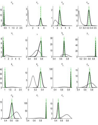
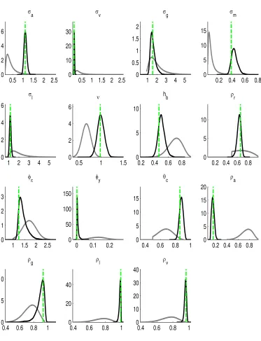
The plots of the prior and posterior distributions of the parameter estimates under all the models are given in Figures (4)-(6).

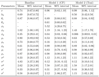
All the parameters are estimated to be significantly different from zero. Moreover, most of the behavioral parameter estimates are similar across the three model specifications. The key findings are as follows. Focusing on the preference parameters of the baseline model, the estimated value of the labor elasticity parameter ν is 0.74 which implies that the Frisch elasticity is around 1.35. This value is higher than 1.00 as implied by the other two model specifications. Both the baseline and Model 2 specifications estimate the intermediate habit persistence hb (0.69 and 0.50, respectively) which is consistent with Smets and Wouters

8

(2007).

The estimate of the price stickiness parameterθc in the baseline case is around 0.87 and

is quite close to the other two estimates (0.89, Model 1; 0.88, Model 2). This implies that the average duration of the price contract in all the three models is around 7.69 quarters, which is much longer than the 3 quarters found in Smets and Wouters (2007). Furthermore, the average duration of the wage contract implied by Model 1 is 2.56 (θw = 0.61) which is

consistent with other related studies (Smets and Wouters (2007), Justiniano, Primiceri and Tambalotti (2010, 2011)). Finally, the elasticity of the cost of changing the stock of durables

φ1 in Model 1 is estimated to be higher than its prior mean, around 5.52, implying an even slower response of the stock of durables to any exogenous shocks.

Turning to the estimates of the parameters governing the exogenous shocks, a few points are worth mentioning. First, both the intratemporal preference shocks and relative price shocks are estimated to be very persistent in all three specifications. Second, the absence of hump-shaped endogenous dynamics induced by internal habits is compensated by more persistent and volatile intertemporal preference shocks in Model 1. Third, while the estimate of the standard deviation of the relative price shock in the baseline case is around 4.83 and is higher than the estimates in other specifications, that of the neutral technology shock in the baseline model is somewhat lower than that in the other two models. The small wealth effect implied by the augmented GHH preferences induces a strong transmission mechanism for the relative price shocks.9 _{Finally, the estimated means of the standard deviation of the}

monetary policy shocks are similar in all three cases (0.33, baseline; 0.31, Model 1; 0.44, Model 2).

The estimate of the interest rate smoothing parameter (0.90) is somewhat higher in the baseline model compared to the other two models (0.53, 0.63), indicating a considerable de-gree of smoothing. The mean of the long-run reaction coefficient to inflation is comparable across the models. However, the authorities do not appear to react very strongly to the output gap level in the short-run in any of the models.

6.2

Impulse Responses

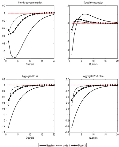
Recall that our estimation exercise has two goals: to examine how well each estimated model can (i) explain the co-movement puzzle, and (ii) fit the data. To pursue the first goal, we plot the impulse responses of key variables to a (one standard deviation) monetary policy shock computed at the estimated posterior means of the parameters as given in Figure (7).

9

We observe that all three estimated models can resolve the co-movement puzzle. However, the internal propagation mechanisms differ across the three models.

In the baseline case, aggregate hours fall due to the small wealth effect on labor sup-ply after a contractionary monetary policy shock (solid line in Figure (7)). This induces a fall in both durable and non-durable production, confirming our intuition from the calibra-tion exercise in Seccalibra-tion (2). Furthermore, internal habit persistence generates hump-shaped responses in non-durable consumption, making it less interest-sensitive than durable con-sumption which is consistent with the empirical VAR findings.

Model 1 introduces nominal wage stickiness in the standard sticky price model as in Carlstrom and Fuerst (2006). Given that labor is the only input, stickiness in nominal wages induces stickiness in the durable goods prices. Hence, durable goods producers have little incentive to adjust their prices as long as the wages are sticky. This causes the aggregate labor, aggregate production, non-durables and durables to fall after a contractionary policy shock (dashed-dot line in Figure (7)). Furthermore, the introduction of adjustment costs prevents the responses of durable goods consumption from moving in the opposite direction after the initial fall on impact.

Finally Model 2 explores the role of the financial frictions as in Tsai (2010). The intro-duction of a working capital channel imposes the firms to borrow in advance in order to pay wages. After a contractionary monetary policy shock, the marginal cost rises, discouraging production in both the durable and non-durable goods sectors, and thereby inducing a fall in the aggregate labor. Finally, the consumption smoothing motive implied by habit formation dampens the response of non-durable goods consumption to the shock (dashed-star line in Figure (7)).

6.3

Model Fit

In this section, we achieve the second goal of the estimation exercise by comparing the models’ fit. One advantage of Bayesian analysis is that it can be employed to assess the relative plausibility of alternative model specifications by comparing the log marginal likelihood.10

Table 4 reports the out-of-sample forecasts under each specification. The marginal likelihoods are based on Geweke’s Harmonic Mean Estimator. Column 3 reports Bayes’ factor which is the difference between the log marginal likelihood in alternative cases and the baseline case. The smaller is the number, the stronger is the evidence in favor of the baseline case.

10

It is quite evident that the data strongly favor Model 2 over all the specifications followed by Model 1. The marginal log-likelihood under Model 1 and Model 2 increases by 121 and 214, respectively, compared to the baseline model, which means that priors that favor the baseline model over Model 1 and Model 2 by factors of 7.6×1052 _{and 8.6×10}92 _{are needed}

in order to accept it after observing the data. These factors are very high, and so the data strongly reject the baseline model compared to the other cases.

In a nutshell, there are key structural differences across the three models that affect the reduced form dynamics of durable consumption, non-durable consumption, hours, inflation and the interest rate and hence the models’ overall fit to the actual data. Our findings suggest that Model 2 with a working capital channel not only successfully resolves the co-movement puzzle, but also outperforms the other two specifications in fitting the data.

7

Conclusion

References

[1] Barsky, Robert, Christopher House, and Miles Kimball, “Sticky Price Models and Durable Goods,” American Economic Review 97(3), pp. 984-998, 2007.

[2] Calvo, G., “Staggered Prices in a Utility Maximizing Framework,”Journal of Monetary Economics, 1983.

[3] Carlstrom, Charles and Timothy Fuerst, “Co-movement in Sticky Price Models with Durable Goods.” Federal Reserve Bank of Cleveland Working Paper 06-14, 2006.

[4] Christiano, L., M. Eichenbaum, and C. Evans, “Nominal Rigidities and the Dynamic Effects of a Shock to Monetary Policy,”Journal of Political Economy, vol. 113 (1), 1-45, 2005.

[5] Engel, C. and J. Wang, “International Trade in Durable Goods: Understanding Volatil-ity, Comovement, and Elasticities,”Journal of International Economics 83(1), 37-52, 2011.

[6] Erceg, Christopher and Andrew Levine, “Optimal Monetary Policy with Durable Con-sumption Goods.” Journal of Monetary Economics 53, pp. 1341-1359, 2006.

[7] Fern´andez-Villaverde, J. and J.F. Rubio-Ram´ırez, “Comparing Dynamic Equilibrium Models to Data: A Bayesian Approach,” Journal of Econometrics Vol. 123, pages 153 - 187, 2004.

[8] Greenwood, J., Z. Hercowitz and G. W. Huffman, “Investment, Capacity Utilization and the Real Business Cycle,” American Economic Review, 78, 402-17, 1988.

[9] Ichiue, H., T. Kurozumi, and T. Sunakawa, “Inflation Dynamics and Labor Adjustments in Japan: A Bayesian DSGE Approach,” Economic Enquiry, forthcoming.

[10] Jaimovich, N. and S. Rebelo, “Can News about the Future Drive the Business Cycle?”

American Economic Review, vol-99, issue 4, pages 1097-1118, 2009.

[11] Justiniano, A., G. Primiceri and A. Tambalotti, “Investment Shocks and Business Cy-cles,” Journal of Monetary Economics, 57(2), 132-145, 2010.

[13] Kim, K.H. and Katayama, M., “Intertemporal Substitution and Sectoral Comovement in a Sticky Price Model,” Departmental Working Papers 2010-01, Department of Eco-nomics, Louisiana State University, 2011.

[14] King, R.G. and S. Rebelo, “Resuscitating Real Business Cycles”, in J. Taylor and M. Woodford (eds), Handbook of Macroeconomics, North Holland, 927-1007, 2000.

[15] King, Robert G., C. Plosser, and S. Rebelo, “Production, Growth and Business Cycles: I. the Basic Neoclassical Model,” Journal of Monetary Economics, 21: 195-232, 1988.

[16] Kitamura, K. and T. Takamura, “Can Sticky Information Solve Comovement Problem in Two-Sector Model with Durable Goods,” working paper, 2010.

[17] Levin, A. and T. Yun, “Durable Goods and Persistent Recession,” manuscript, Federal Reserve Board, 2011.

[18] Lubik, T. A. and F. Schorfheide, “A Bayesian Look at New Open Economy Macroe-conomics,” edited by Mark, G. and Rogoff, K., NBER Macroeconomics Annual 2005, Volume 20, pages 313-382, 2006.

[19] Monacelli, T. and R. Perotti, “Fiscal Policy, Wealth Effects, and Markups,” Working Paper 14584, NBER Working Paper Series, 2008.

[20] Rabanal, P. and J.F. Rubio-Ram´ırez, “Comparing New Keynesian Models in the Euro Area: A Bayesian Approach,” Journal of Monetary Economics, Vol. 52, pp. 1151-1166, September 2005.

[21] Rabanal, P. and V. Tuesta, “Euro-Dollar Real Exchange Rate Dynamics in an Estimated Two-Country Model: An Assessment,” Journal of Economic Dynamics and Control, Vol. 34, April, pp. 780-797, 2010.

[22] Raffo, A., “Net Exports, Consumption Volatility and International Business Cycle Mod-els,” Journal of International Economics, 75, 14-29, 2007.

[23] Raffo, A., “Technology Shocks: Novel Implications for International Business Cycles,” Board of Governors of the Federal System, manuscript, 2009.

[25] Smets, F. and R. Wouters, “An Estimated Dynamic Stochastic General Equilibrium Model of the Euro Area,” Journal of European Economic Association, Vol. 1(5): 1123-1175, 2003.

[26] Smets, F. and R. Wouters, “Shocks and Frictions in US Business Cycles: A Bayesian Approach,” European Central Bank, working paper, No. 722, 2007.

[27] Sudo, N., “Sectoral Co-Movement, Monetary-Policy Shock, and Input-Output Struc-ture,” IMES Discussion Paper Seies 08-E-15, Institute for Monerary and Economic Studies, Bank of Japan, 2008.

TECHNICAL APPENDIX

A

Household’s problem

U(Ct, Dt, Nt) =ǫgt

(Bt)−ǫltφNt1+νHt

s.t.

Ht=H(1 −γ) t−₁ (Bt)

γ

whereBt= (Ct−hbCt−1)ψcDtψd andǫ g

t, ǫlt are preference shock and labor-preference shock

respectively. Then the household optimization problem is:

M axXβtU(Ct, Dt, Nt) 1−σ

1−σ

s.t.

Pc,tCt+Px,tXt+Px,t

1 2φ1

(Xt−δDt−₁)2

Dt−1

≤WtNt+ Πt+Tt+St−₁−

St

Rt

, t= 0,1, .. (1)

Ht=H(1 −_γ) t−₁ (Bt)

γ

(2)

Dt= (1−δ)Dt−₁+X_t (3)

Let Λt,Ωt,Ξtrepresent the langrangian multipliers for constraints (1) (2) and (3) respectively.

The household foc with respect to Ct, Xt, Dt, Nt, Ht are:

Λt=ψcU −_σ t

Bt

(Ct−hbCt−₁)

ǫgt−hbβψcEt

U−_σ

t+1ǫ

g t+1

Bt+1

(Ct+1−hbCt)

+γψcΩtH1 −_γ t−₁ (Bt)

γ−1 Bt

(Ct−hbCt−₁)

−hbβγψcEt

Ωt+1(Bt+1)γ

−₁

H1−_γ t

Bt+1

(Ct+1−hbCt)

(4)

Λt

Px,t

Pc,t

+ Λt

Px,t

Pc,t

φ1(Xt−δDt−1) Dt−1

Ξt−β(1−δ)EtΞt+1 =ψdU −_σ t

Bt

Dt

ǫg_t +γψdΩtH(1 −γ) t−₁

(Bt)γ

Dt

+ Λt

Px,t

Pc,t

" φ1δ

(Xt−δDt−₁)

Dt−₁

+φ1 2

(Xt−δDt−₁)

2 D2

t−₁

#

(6)

U−_σ

t φ(1 +ν)NtνHtǫgtǫlt= Λt

Wt

Pc,t

(7)

Ωt+U −σ

t φNt1+νǫ g

tǫlt=β(1−γ)EtΩt+1(Bt+1)γH

−γ

t (8)

Detrend: To detrend our model, let Bt = btAtZtϕd, Ht = htAtZtϕd, BCtt =

bt

ct

(Zt)ϕd, Bt

Dt =

bt dt 1 Zt ϕc

, U(.)−σ

= (At) −σ

(Zt)ϕd( −σ)

u(.)−σ

, Λt = (At) −σ

(Zt)ϕd(1 −σ)

λt, Ωt =

(AtZtϕd) −_σ

ωt, Ξt = ξt(At) −_σ

(Zt)ϕd(1 −_σ)−₁

Wt = Atwt, P_Pxt_ct = _Z1_tp_pxt_ct, then we can have the

following equations.

λt =ψcu −_σ t

bt

(ct−hbct−1/g_a,t)

ǫgt −hbβψcEt

h u−_σ

t+1g

−_σ a,t+1g

ψd(1−σ)

z,t+1 ǫ

g t+1

i _bt+1

(ct+1−hbct/ga,t+1)

+γψcωt

h1−_γ t−₁b

γ t

(ct−hbct−1/ga,t)

h ga,tgψz,td

iγ−1

−hbβγψcωt+1

bγ_t+1h1−_γ t

(ct+1−hbct/ga,t+1)

g−_σ+γ−₁ a,t+1 (g

ψd

z,t+1)1

−_σ+γ−₁

(D.1)

λt

px,t

pc,t

+λt

px,t

pc,t

φ1(ga,tgz,txt−δdt−1)

dt−₁

=ξt (D.2)

ξt−λt

px,t

pc,t

φ1(ga,tgz,txt−δdt−₁)

δ dt−1

+1

2φ1(ga,tgz,txt−δdt−1)

2 1 d2

t−₁

−β(1−δ)Etξt+1g −_σ a,t+1g

ψd(1−σ)−1

z,t+1

=ψdu−tσ

bt

dt

ǫg_t +γψdωth(1 −_γ) t−₁

(bt)γ

dt

[ga,tgz,tψd]γ −1

(D.3)

u−σ

t φ(1 +ν)Ntνhtǫgtǫlt=λt

wt

Pc,t

(D.4)

ωt+u −_σ

t φNt1+νǫ g

tǫlt =β(1−γ)Etωt+1(ga,t+1gz,tψd+1)γ

−_σ

(bt+1)γh

−_γ

Non-durable goods firms optimization problem gives:

M Cc,t=

Wt

At

(A.1)

Durable goods firms optimization problem gives:

M Cx,t =

Wt

ZtAt

(A.2)

M Cx,t =Px,t (A.3)

Combining (A.1) and (A.2):

M Cx,t

M Cc,t

= 1

Zt

= Px,t

Pc,t

Steady state: From (D.5),

ω= u

−σ

φN1+ν

β(1−γ)−1 (ss.1) From D.1,

λ = ψcu

−_σ

b c(1−hb)

(1−βhb)

1 + γφN

1+ν

β(1−γ)−1

(ss.2)

From D.2,

λ=ξ (ss.3)

From D.3 and ss.1

ξ[1−β(1−δ)] = ψdu −_σb

d

1 + γφN

1+ν

β(1−γ)−1

(ss.4)

From ss.2, ss.3 and ss.4,

ψc =

c/d

1−_β(1−_δ)

1−_βhb

1−_hb + c/d

1−_β(1−_δ)

From D.4 and ss.4

φ =

ψdb/d

1−_β(1−_δ)

N1+νh(1+ν)h/N

(ǫ−_1)/ǫ −

ψd(b/d)γ

(1−_β(1−_δ))(β(1−_γ)−₁₎

Log-linearize:

(1−_βhb)ˆλt= (β(1

−_γ)−₁₎

(β(1−_γ)−_{1) +γφN}1+ν

−_{σuˆt+ ˆbt}− 1

1−_hb(ˆct −_hbˆct

−1+hbgˆa,t) + ˆǫgt

− hbβ(β(1

−_γ)−₁₎

(β(1−γ)−1) +γφN1+ν

−σuˆ_t+1−σˆg_a,t+1+ψ_d(1−σ)ˆg_z,t+1+ ˆb_t+1− 1

1−h_b(ˆct+1

−h_bˆc_t+h_bˆg_a,t+1) + ˆǫg_t+1

+ γφN

1+ν

β(1−γ)−1 +γφN1+ν

ˆ

ωt+ (1−_{γ)ˆht−1+γ}ˆ_bt− 1

1−h_b(ˆct

−_{hbˆct−1+hbˆga,t) + (γ}−_{1)(ˆga,t+ψdˆgz,t)}

− hbβγφN

1+ν

β(1−_γ)−_{1 +γφN}1+ν

ˆ

ωt+1+ (1−_γ)ˆht+γˆ_bt+1− 1

1−_hb(ˆct+1

−_{hbˆct+hbˆga,t+1) + (}−_σ+γ−_{1)ˆga,t+1+ (1}−_σ+γ−_{1)ψdˆgz,t+1}

(L.1) ˆ

λt+ ˆpx,t−_{pˆc,t+φ1δ(ˆxt}−_dˆ_t

−1+ ˆga,t+ ˆgz,t) = ˆξt (L.2)

ˆ

ξt−φ₁δ2(ˆxt−dˆ_t−1+ ˆga,t+ ˆgz,t)−β(1−δ) h

ˆ

ξt+1−σˆg_a,t+1+ (ψ_d(1−σ)−1)ˆg_z,t+1 i

= (1−β(1−δ))(β(1−γ)−1) (β(1−_γ)−_{1) +γφN}1+ν (

−σuˆt+ ˆbt−dˆt+ ˆǫg_t)

+ (1−β(1−δ))γφN

1+ν

(β(1−γ)−1) +γφN1+ν h

ˆ

ωt+ (1−_{γ)ˆht−1+γ}ˆ_bt−_dˆ_{t+ (γ}−_{1)(ˆga,t+ψdgˆz,t)} i

(L.3)

1

β(1−_γ) h

ˆ

ωt+ (β(1−γ)−1)(−σuˆt+ (1 +ν) ˆNt+ ˆǫg_t + ˆǫlt)

i

= ˆωt+1+ (γ−σ)(ˆg_a,t+1+ψ_dˆg_z,t+1) +γ(ˆb_t+1−ˆht) (L.4)

ˆ

λt+ ˆwt−_pˆc,t=−_σuˆt+νNˆ_{t+ ˆht+ ˆǫ}g

t + ˆǫlt (L.5)

ˆ

ht= (1−_γ)ˆht

−1+γˆbt+ (γ−_{1)(ˆga,t+φdgˆz,t) (L.6)}

ˆ_bt= ψc

1−h_b(ˆct

−h_bˆc_t−1+h_bˆg_a,t) +ψ_ddˆ_t (L.7)

ˆ

ut=

1 (1−_φN1+ν₎

h

ˆ

bt−_φN1+ν_{((1 +ν) ˆNt+ ˆh+ ˆǫ}l_t) i

(L.8)

Alternative Specifications:

• Baseline (Augmented GHH): φ1 = 0, γ = 0

• Model 1: hb = 0, γ = 1

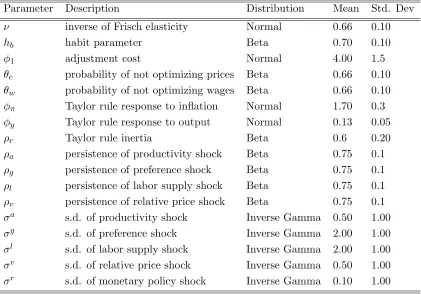
Table 2: Priors of structural parameters

Parameter Description Distribution Mean Std. Dev

ν inverse of Frisch elasticity Normal 0.66 0.10

h_b habit parameter Beta 0.70 0.10

φ1 adjustment cost Normal 4.00 1.5

θc probability of not optimizing prices Beta 0.66 0.10

θw probability of not optimizing wages Beta 0.66 0.10

φπ Taylor rule response to inflation Normal 1.70 0.3

φy Taylor rule response to output Normal 0.13 0.05

ρr Taylor rule inertia Beta 0.6 0.20

ρa persistence of productivity shock Beta 0.75 0.1

ρg persistence of preference shock Beta 0.75 0.1

ρl persistence of labor supply shock Beta 0.75 0.1

ρv persistence of relative price shock Beta 0.75 0.1

σa s.d. of productivity shock Inverse Gamma 0.50 1.00

σg s.d. of preference shock Inverse Gamma 2.00 1.00

σl s.d. of labor supply shock Inverse Gamma 2.00 1.00

σv s.d. of relative price shock Inverse Gamma 0.50 1.00

σr s.d. of monetary policy shock Inverse Gamma 0.10 1.00

Notes: This table lists the description and prior distributions of the structural parameters. The parameters

θw and hare only used in Model 1 and Model 2 respectively. All the other parameters are used in all the

Table 3: Posterior of structural parameters

Baseline Model 1 (CF) Model 2 (Tsai) Parameters Mean 90% interval Mean 90% interval Mean 90% interval

ν 0.74 [0.67,0.80] 0.96 [0.82,1.10] 0.99 [0.86, 1.12]

hb 0.69 [0.67,0.72] - - 0.50 [0.42,0.58]

θc 0.87 [0.86,0.87] 0.89 [0.88,0.91] 0.88 [0.84, 0.92]

θw - - 0.61 [0.60,0.62] -

-φ1 - - 5.52 [4.20,6.75] -

-φπ 1.02 [1.00,1.05] 1.19 [1.16, 1.23] 1.43 [1.17,1.70]

φy 0.35 [0.29,0.41] 0.04 [0.03, 0.06] 0.006 [0.0010, 0.01]

ρr 0.90 [0.89,0.92] 0.53 [0.50,0.56] 0.63 [0.57,0.69]

ρa 0.73 [0.68,0.77] 0.16 [0.11,0.20] 0.15 [0.11,0.18]

ρg 0.61 [0.55,0.68] 0.99 [0.98,0.99] 0.89 [0.82, 0.96]

ρl 0.97 [0.96,0.98] 0.83 [0.79, 0.85] 0.98 [0.96,0.99]

ρv 0.97 [0.96,0.97] 0.98 [0.98,0.99] 0.95 [0.93,0.97]

σa 0.33 [0.28,0.37] 1.12 [1.01,1.23] 1.11 [1.00,1.22]

σv 4.83 [4.37,5.30] 0.12 [0.10, 0.13] 0.12 [0.10,0.14]

σg 2.62 [2.28,2.95] 7.58 [3.97,11.22] 1.58 [1.17,2.01]

σr 0.33 [0.28,0.37] 0.31 [0.27, 0.34] 0.44 [0.36,0.52]

σl 0.58 [0.48,0.67] 2.12 [1.86,2.37] 1.15 [1.02,1.28]

Notes: This table lists the prior distributions of the structural parameters in all the three estimated models: baseline, Model 1 and Model 2. The two numbers in the parentheses are the 90% confidence intervals.

Table 4: Marginal Likelihood

Model Log Marginal Likelihood Bayes’ Factor Baseline -1262.283 0

Model 1 -1140.516 121.767 Model 2 -1048.170 214.113

0 5 10 15 20 -1.5

-1 -0.5 0 0.5 1 1.5 2 2.5 3

Quarters Non-durable consumption

GHH Standard

0 5 10 15 20

-1.5 -1 -0.5 0 0.5 1 1.5 2 2.5 3

Durable consumption

Quarters

0 5 10 15 20

-1.5 -1 -0.5 0 0.5 1 1.5 2 2.5 3

Aggregate Hours

Quarters

0 5 10 15 20

-1.5 -1 -0.5 0 0.5 1 1.5 2 2.5 3

Aggregate Production

Quarters

Labor   LS  

LD   Real  Wage  

W*/P  

L*(BHK)   L’  (GHH)  

W’/P  

1970 1975 1980 1985 1990 1995 2000 -6

-4 -2 0 2 4

log(N)

1970 1975 1980 1985 1990 1995 2000 -10

-5 0 5

Δlog(X)

1970 1975 1980 1985 1990 1995 2000 -2

-1 0 1

Δlog(C)

1970 1975 1980 1985 1990 1995 2000 -3

-2 -1 0 1 2 3

Δlog(P)

1970 1975 1980 1985 1990 1995 2000 -1

0 1 2

R

0.5 1 1.5 2 2.5 0 5 10 15 σ_a

2 4 6

0 1 2 3

σ_v

1 2 3 4 5

0 1 2

σ_g

0.1 0.2 0.3 0.4 0.5 0

5 10 15

σ_m

1 2 3 4 5

0 2 4 6 8 σ l

0.4 0.6 0.8 0

5 10

ν

0.4 0.6 0.8

0 10 20 30 h b

0.2 0.4 0.6 0.8 0 20 40 60 ρ r

1 1.5 2 2.5

0 10 20 30 40 φ_π

0 0.2 0.4

0 5 10

φ y

0.4 0.6 0.8

0 50 100

θ c

0.4 0.6 0.8

0 5 10 15 ρ a

0.4 0.6 0.8 0

5 10

ρ g

0.4 0.6 0.8 0

50 100

ρ l

0.4 0.6 0.8 0 5 10 15 ρ v

0.5 1 1.5 2 2.5 0 2 4 6 σ_a

0.5 1 1.5 2 2.5 0

20 40

σ_v

0 10 20

0 0.2 0.4 0.6 0.8 σ_g

0.1 0.2 0.3 0.4 0.5 0 5 10 15 20 σ_m

1 2 3 4 5

0 1 2 3 σ l

0.5 1 1.5

0 2 4

ν

0 5 10

0 0.2 0.4 0.6 φ 1

0.2 0.4 0.6 0.8 0

10 20

ρ r

1 1.5 2 2.5

0 5 10 15 20 φ_π

0 0.1 0.2

0 20 40

φ y

0.4 0.6 0.8 0 20 40 60 θ c

0.4 0.6 0.8

0 50 100

θ w

0.2 0.4 0.6 0.8 0 5 10 15 ρ a

0.4 0.6 0.8 1

0 50 100 150 ρ g

0.4 0.6 0.8

0 10 20

ρ l

0.4 0.6 0.8 1

0 50 100

ρ v

0.5 1 1.5 2 2.5 0 2 4 6 σ_a

0.5 1 1.5 2 2.5 0

10 20 30

σ_v

1 2 3 4 5

0 0.5 1 1.5 2 σ_g

0.2 0.4 0.6 0.8 0

5 10 15

σ_m

1 2 3 4 5

0 2 4 6 σ l

0.5 1 1.5

0 2 4 6

ν

0.2 0.4 0.6 0.8 0

5 10

h b

0.2 0.4 0.6 0.8 0

5 10

ρ r

1 1.5 2 2.5 0

1 2 3

φ_π

0 0.1 0.2

0 50 100 150 φ y

0.4 0.6 0.8 1 0 5 10 15 θ c

0.2 0.4 0.6 0.8 0 5 10 15 20 ρ a

0.4 0.6 0.8 1 0

5 10

ρ g

0.4 0.6 0.8 1

0 20 40

ρ l

0.4 0.6 0.8 1

0 10 20 30 40 ρ v

0 5 10 15 20 -1.2

-1 -0.8 -0.6 -0.4 -0.2 0 0.2

Quarters Non-durable consumption

Baseline Model 1 Model 2

0 5 10 15 20

-4 -3 -2 -1 0 1 2

Durable consumption

Quarters

0 5 10 15 20

-1.6 -1.4 -1.2 -1 -0.8 -0.6 -0.4 -0.2 0 0.2

Aggregate Hours

Quarters

0 5 10 15 20

-1.6 -1.4 -1.2 -1 -0.8 -0.6 -0.4 -0.2 0 0.2

Aggregate Production

Quarters

Figure 7: Estimated mean impulse responses from monetary policy shock.