Chaos Behavior and Estimation of the Unknown Parameters of Stochastic Lattice Gas for Prey Predator Model with Pair Approximation

(1)

http://www.scirp.org/journal/am ISSN Online: 2152-7393

ISSN Print: 2152-7385

Chaos Behavior and Estimation of the Unknown

Parameters of Stochastic Lattice Gas for

Prey-Predator Model with Pair-Approximation

Saba Mohammed Alwan

Department of Mathematics and Computer Science, Faculty of Science, Ibb University, Ibb, Yemen

Abstract

In this paper, the problem of chaos, stability and estimation of unknown parameters of the stochastic lattice gas for prey-predator model with pair-approximation is stu-died. The result shows that this dynamical system exhibits an oscillatory behavior of the population densities of prey and predator. Using Liapunov stability technique, the estimators of the unknown probabilities are derived, and also the updating rules for stability around its steady states are derived. Furthermore the feedback control law has been as non-linear functions of the population densities. Numerical simula-tion study is presented graphically.

Keywords

Stochastic Lattice Gas Model, Prey-Predator, Updating Rules, Estimation, System State

1. Introduction

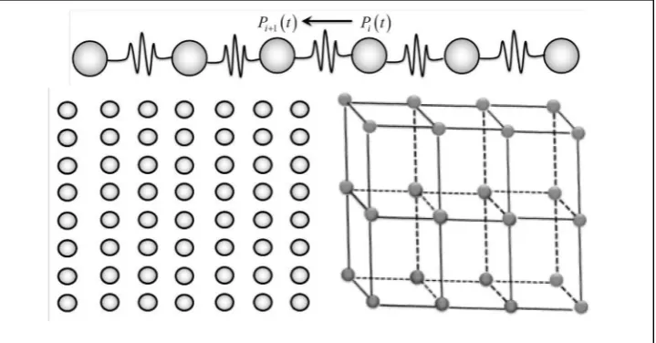
A lattice model usually represents the motion of a network of particles, where the mo-tion is produced by forces acting between the neighboring particles. Lattice models also are used to simulate the structure of polymers and can exhibit its dynamic behaviors.

The interaction between particles of the systems, which is the subject of this study, is continuous-time Masrkov process on certain spaces of configurations of particles. These systems began as a branch of probability theory in the 1960’s. Most of the inputs came from the work of Spitzer in United States [1] and of Dobrushin in the Soviet Un-ion [2]. From a mathematical point of view, interacting particles systems represent a natural departure from the established theory of Markov processes. The lattice can be in one, two, three or complex dimensions. The one-dimensional lattices consider a li-near arrangement between the sequences of particles, and each particle connected to How to cite this paper: Alwan, S.M. (2016)

Chaos Behavior and Estimation of the Un-known Parameters of Stochastic Lattice Gas for Prey-Predator Model with Pair-Approxi- mation. Applied Mathematics, 7, 1765-1779.

http://dx.doi.org/10.4236/am.2016.715148

Received: August 1, 2016 Accepted: September 18, 2016 Published: September 21, 2016

http://creativecommons.org/licenses/by/4.0/

(2)

the next one by a spring depends upon a condition. There are many classifications for the two-dimension lattice, such as a centered rectangular lattice, a hexagonal lattice, square lattice and so on (see Figure 1).

Many of models of interacting particles system have shown a chaos behavior. The problems of estimating and controlling stochastic systems are far from solved, and a considerable amount of research is under way. Estimation of the internal states of a stochastic dynamical system is a topic with important applications in different fields such as physics, biology and medicine [3]-[5].

A spatial stochastic model to discuss strategies to control the epidemic was intro-duced by Schinazi [6]. El-Gohary has proposed a stochastic model to study the problem of optimal controlling the epidemic [3][4]. El-Gohary and Al-Ruziza have suggested a non-linear stochastic model to investigate the optimal control of a non-homogenous prey-predator model. They have derived the feedback control law as non-linear func-tions of the population densities [7][8]. El-Gohary has studied the problems of chaos and optimal control cancer model with complete unknown parameters [9]. Al-Mahdi and Khirallah have studied stability and bifurcation analysis of a model of cancer [10] [11]. Alwan and El-Gohary have studied the chaos, estimation and optimal control of habitat destruction model and genital herpes epidemic models with uncertain para-meters [12][13].

[image:2.595.195.555.488.676.2]

A stochastic lattice gas model is proposed to describe the dynamics of two animals populations, one being a prey and the other a predator [14]. El-Gohary and Alwan have discussed the problem of chaos and control of a stochastic lattice gas model for prey- predator when one-site approximation is used. They have studied stability of the system and derived the optimal control inputs. They have also derived the estimators of the un-known parameters and probabilities [15]. This paper is considered as an extension of the paper [15] where it will discuss the stability and estimation of the unknown parameters of the stochastic lattice gas model for prey-predator when two-site approximation is used.

(3)

This paper has the following structure. In section 2, the stochastic probability model and its proposed rules will be discussed, and also the pair approximation mathematical model and its analytical solution will be presented. In section 3, stability analysis of the system will be studied and presented graphically. Estimation of the unknown parame-ters and the updating rules are derived in section 4. In section 5, numerical solutions are derived and presented graphically. Finally, conclusions are provided in Section 6.

2. Stochastic Probability Model

In this section, we will describe the stochastic rules of the proposed stochastic lattice gas model for prey-predator.

The lattice gas models describing special chemical reaction. Let us consider a lattice of N sites, every site can be either empty (O) or occupied by a prey (1) or occupied by a predator (2). At any time step a site is randomly chosen. For that site, we suppose that

1

n and n2 are the numbers of the nearest neighbors of that site occupied by prey or

predator, respectively and S is the total number of nearest neighbors of this site. The transition matrix of the model is given in Table 1 or graphically in Figure 2.

This Markov process contains three probability parameters p1, p2 and p3, which

are associated to the process: birth of prey process, death of prey and simultaneous birth of predator, and spontaneous death of the predator [14]-[17]. The parameters

1

p, p2 and p3 satisfy the condition:

Table 1. The transition matrix of the model.

O 1 2

O 1−p n S1 1 p n S11 0

1 0 1−p n S2 2 p n S2 2

[image:3.595.195.555.404.705.2]

2 p3 0 1−p3

(4)

1 2 3 1

p +p +p = . (1)

Let us consider the system state as µ=

(

µ µ1, 2,,µN

)

where µ =i,i 0,1 or 2

ac-cording whether the state i empty, occupied by prey or occupied by predator respectively. Let P

( )

µ,t be the probability of the state μ at time t. The time evolution of the proba-bility of the state μ P

( )

µ,t and the mathematical system is given in details in [14]. The final mathematical expression of the model is a hierarchical system of equations, where the one-site correlations Pi

( )

θ1 involve the two-site correlations Pij

(

θ θ1 2

)

and the

two-site correlations involve three-site correlation Pijk

(

θ θ θ1 2 3

)

and so on, where θ θ1, 2

and θ3 take one values of 0, 1, or 2 (see Equation (6) in [14]). The mean field

ap-proximation theory is used to derive a closed set of equations. The one-site approxima-tion of this hierarchical system of Equaapproxima-tion (6) in [14] is accomplished by writing the two-site correlation Pij

(

θ θ1 2

)

as the product Pi

( ) ( )

θ1 Pj θ2 in the hierarchical system.

The two-site approximation model which is the subject of this paper will be discussed in the next section.

Pair Approximation Mathematical Model

In this section, the two-site approximation will be presented and the final mathematical model will be written.

In the hierarchical system Equation (6) in [14], the mean field theory is suggest an ap-proximation to derive a closed set of equations as: The thee-site correlations Pijk

(

θ θ θ1 2 3

)

can be expressed in terms of two-site and one-site correlations as follows

(

1 2

)

( ) ( )

ij i j

P θ θ ≈P θ P θ (2)

(

)

(

1 2

) (

_{( )}

2 3

)

1 2 3

2

ij jk

ijk

j

P P

P

θ θ θ θ θ θ θ

θ

≈ ₍₃₎

where sites i and k are the nearest neighbors of site j. We also seek for spatially homo-geneous and isotropic solutions of Equation (6) in [14]. In this case we may drop the indexes in Pi

( )

θ1 and Pij

(

θ θ1 2

)

. We then have three one-site correlations

( )

, 0,1 or 2

i

P θ θ= , and nine two-site correlations P_ij

( )

θϕ θ ϕ, , =0,1 or 2, which are presented in the transition matrix in Table 1. However, only five of them are indepen-dent. We choose them to be P

( )

1 =x (the prey density), P

( )

2 =y (the predator density), P

( )

3 =P

( )

01 =u, P

( )

12 =P

( )

4 =v, and P

( )

02 =P

( )

5 =w. Let us con-sider also P

( )

0 = = − −z 1 x y (the vacuum site density). The equations for these va-riables and the final mathematical system according this pair approximation are given by:

( )

1

( )

2

( )

d

1 3 4 ,

dtP = p P −p P

(4a)

( )

2

( )

3

( )

d

2 4 2

dtP = p P −p P ,

(4b)

( )

1

( )

2

( )

2

( ) ( )

_{( )}

3

( )

1

( )

3 3 3 4 3

d 1

3 4

d 1

qP P P P P

S

P p p p P p

t S z P S

 − 

−

= _ − _+ −

(5)

( )

1

( ) ( )

2

( )

_{( )}

2

( )

2

( )

3

( )

3 5 4 4 4

d 1

4 4

d 1

P P rP P P

S

P p p p p P

t S z P S

 − 

−

= _ + _− −

  , (4d)

( )

2

( ) ( )

_{( )}

1

( ) ( )

3

(

( )

)

3 4 3 5

d 1

5 5

d 1

P P P P

S

P p p p l P

t S P z

 

−

= _ − _+ −

  , (4e)

where

( )

0 1 1 2 ,

00 3 5 ,

11 1 3 4 ,

22 2 4 5

z P P P

q P z P P

r P P P P

l P P P P

= = − − 



= = − − _



= = − − _



= = − − _

(5)

and S is the total number of nearest neighbors of the site. This is a nonlinear system of differential equations. The analytical solution for this system is given by solving the system of equation:

( )

d

0, 1, 2, , 5

dtP i = i=  . (6) By Maple program and [14], when S=4, the system in Equation (6) has the

fol-lowing general solution

( )

(

)

1

1 1 3 1 1 2 1 1

1 1 2 1

P = +u p p + u α α+ − β + u − , (7a)

( )

2 1

( )

1 1 3

P =p P u p , (7b)

( )

3

( )

1 1

P =P u , (7c)

( )

4

( )

1 1 1 2

P =P u p p ,

(7d)

( ) (

5 1 1 2

)

₍

1

( )

1

( )

2

₎

P = βu −α −P −P , (7e)

where,

(

)

(

)

(

)

1 p S3 p2 S 2 p2 S 1 ,

α = + − − α =2

(

p2

(

S− −2

)

p S3

)

p2

(

S−1 ,

)

1 1 2p1 p2,

β = + β₂ =2Sp₃ p S₁

₍

−1 ,

₎

(

)

(

₂ 1 2

)

1 4 2 ,

u = B− B − AC A A=

(

β1−1

)(

β1+1 ,

)

(

2

)(

1 1

) (

1 1

)(

1 2

)

2 1 2,

B= γ α+ β + + β − α α+ + β β

(

2

)(

1 2

)

2 2 2

C= γ α+ α α+ + β α and γ =s

(

1−p₃ p₂

) (

S−1

)

(for more details, see [14]), and the following two trivial fixed stationary states as special solutions: D1 =

(

z x y u v w, , , , ,

) (

= 1, 0, 0, 0, 0, 0

)

corresponds to the vacuum-absorbing

state, and D2 =

(

z x y u v w, , , , ,

) (

= 0,1, 0, 0, 0, 0

)

corresponds to the prey-absorbing state.

3. Stability Analysis

(6)

some of the equilibrium point will be presented.

For the case of S=2, the system has only special stationary solution which is prey-

absorbing state

(

o x y, ,

) (

= 0,1, 0

)

[14]. This solution is unstable when p2 > p3, and

the general stationary solutions:

(

p2−p3

) (

p1+p3

)

, p3 p2,

(

)

(

)

1 2 3 2 1 3

p p −p _p p +p _ is unstable also, when p2< p3 as in [15]. For the case

4

S= , the system (3) has two trivial fixed stationary states, that are given by:

(

) (

)

1 , , , , , 1, 0, 0, 0, 0, 0

D = z x y u v w = , that correspond to the vacuum-absorbing state, and D2 =

(

z x y u v w, , , , ,

) (

= 0,1, 0, 0, 0, 0

)

, that correspond to the prey-absorbing state.

The Jacobian matrix of the system (4) is given by

11 12 13 14 15 21 22 23 24 25

31 32 33 34 35 41 42 43 44 45 51 52 53 54 55

a a a a a

J a a a a a

a a a a a

        =        

(8) where

11 12 0, 13 1, 14 2, 15 21 0, 22 3, 23 0,

a =a = a = p a = −p a =a = a = −p a =

( )

( ) ( )

( )

( ) ( )

( )

2

24 2 25 31 1 2

2 3 3 5 3 4

1

, 0, ,

1 1 2 1

P P P p P P

S

a p a a p

S P P P

 − −  − = = = _ + _ − −  

( )

( ) ( )

( )

2 32 1

2 3 3 5

1

,

1 1 2

P P P

S

a p

S P P

 − −  − = _ _ − −  

( )

2

( )

1

33 1

1 1 2 4 3 5 4

1

,

1 1 2 1

P P P P p P p

S

a p

S P P P S

 − − − −  − = _ ₋ ₋ − _−  

( )

2 34 3 3 1 , 1 p P S a p S P −  − = _ _+  

( )

1

( )

35 3

3 1

,

1 1 2

p P S

a p

S P P

 −  − = _ _+ − −  

( ) ( )

( )

(

1

)

2

( ) ( )

( )

41 2 2

3 5 3 4

1

, 1

1 1 2

p P P p P P

S a

S _P _P P

  −   = +  ₋ ₋   

( ) ( )

( )

(

1

)

( )

1

( )

2

( )

42 2 43

3 5 5 4

1 1

, ,

1 1 2 1

1 1 2

p P P p P p P

S S

a a

S _P _P S P P P

  _ _ − _ _ − = = _ − _ − −  ₋ ₋  _ _  

( )

2

44 2 3

1 3 4 4

1

, 1

P P P p

S

a p p

S P S

 − − 

−

= _ _− −

 

( )

1

( )

45

3 1

,

1 1 2

p P S

a

S P P

  − = _ ₋ ₋ _  

( ) ( )

( )

₍

_{( )}

( ) ( )

_{( )}

₎

2 1

51 2 2

3 4 3 5

1

,

1 ₁ ₁ ₂

p P P p P P

S a

S P _P _P

₋  −   = −  ₋ ₋   

( ) ( )

( )

(

1

)

52 2 3

3 5 1

,

1 1 2

p P P

S

a p

S _P _P

  −   = − +  ₋ ₋   

( )

2 1 53 4 5 1

1 1 1 2

p P p P

S a

S P P P

− 

−

= _ − _

− −

(7)

( )

2 1

54 3 55 3

3 3

1 1

, 2 .

1 1 1 2

p P p P

S S

a p a p

S P S P P

   − 

− −

= _ _− = _ ₋ ₋ _−

   

The Jacobian matrix in Equation (8) of the system in Equation (4) evaluated at the vacuum-absorbing state D1 is converges to

2 2 1

3 2

1 1 3

3

3 3 3

0 0

0

0 0

0 2

0 2 0

0 0

2

0 0

p p

JD p p

p p

p p p

−

 

 ₋ 

 

≈

 

−

 

 ₋ ₋ 

 

(9)

and its eigenvalues just are the elements of the main diameter, which are

2

1 0, 2 3 0, 3 1 0, 4 3, 5 2 3 0

2

2 p

p p p p

λ = λ = − < λ = > λ = − λ = − < _{. (10)}

Using the linear stability analysis, since λ3 is a positive eigenvalue at least, hence

this stationary solution is absolutely unstable.

Similarly, we get the Jacobian matrix in Equation (8) of the system in Equation (4) evaluated at the prey-absorbing state D2 converges to JD2 =JD1. Accordingly JD2

has the same eigenvalues. Therefore, the stationary state D2 is also absolutely

unsta-ble. The linear stability analysis for these two stationary states indicates sufficiently that, the system of stochastic lattice gas of prey-predator system according to the pair-approximation is absolutely unstable at least in two dimensions. But the stability conditions are requiring more study.

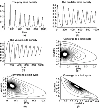
Such behavior for the system in prey, predator and vacuum densities in Figures 3(a)-(c) respectively, represents an oscillatory behavior. For limit-cycle that appear in Figures 3(d)-(f) where all the neighboring trajectories tend to a limit-cycle at time tends to infinity, causing the so-called a stable limit-cycle, which indicates that the sys-tem stochastic lattice gas of prey-predator syssys-tem according to the pair-approximation has an oscillatory behavior.

4. Estimations of the Unknown Probabilities

In this section we will derive the dynamic estimators of the unknown probabilities

1, 2

p p and p3 from the conditions of the asymptotic stability of the system in

Equa-tion (4) about its staEqua-tionary states assistance of some feedback variables.

At the beginning, let us assume the modified model with unknown probabilities in Equation (4) to become as follows

( )

1

( ) ( )

2

( ) ( )

1

d

ˆ ˆ

1 3 4

dtP = p t P −p t P +E (11a)

( )

2

( ) ( )

3

( ) ( )

2

d

ˆ ˆ

2 4 2

dtP = p t P −p t P +E

(11b)

( )

1

( ) ( )

2

( )

2

( ) ( ) ( )

_{( )}

3

( ) ( )

1

( ) ( )

3

3 3 3 4 3

d 1

ˆ ˆ ˆ ˆ

3 4

d 1

qP P P P P

S

P p t p t p t P p t E

t S z P S

 − 

−

= _ − _ + − +

(8)

( )

( ) ( ) ( )

( ) ( )

_{( )}

( )

( ) ( )

2 1

4 2

2 3

3 5 4 4

d 1

ˆ ˆ

4

d 1

4

ˆ ˆ 4

P P rP P

S

P p t p t

t S z P

P

p t p t P E

S

 − 

−

= _ + _

 

− − +

(11d)

( )

( ) ( ) ( )

_{( )}

( ) ( ) ( )

( )

(

( )

)

2

3

1

5

3 4 3 5

d 1

ˆ ˆ

5

d 1

ˆ 5

P P P P

S

P p t p t

t S P z

p t l P E

 

−

= _ − _

 

+ − +

(11e)

where p tˆ_s

( )

are the estimators of the unknown probabilities p_s,

(

s=1, 2, 3

)

and

, 1, , 5

j

E j=  are the control inputs that will be derived to make the trajectory of the system specified by the steady-states D1, D2 and the general solution in Equation (7)

to any of these states. If Ej =0,j=1,, 5, then the system in Equation (11) has an

[image:8.595.199.548.280.660.2]

un-stable special solution:

Figure 3. The densities of the prey, predator and vacuum sites and their limit cycle, respectively for p1=0.49,p2=0.49 and p3=0.02, at the initial densities

| 0 0.25, | 0 0.5, | 0 0.305, | 0 0.29

(9)

( )

, 1, , 5 and ˆ_s

( )

_s,

(

1, 2, 3

)

P j =P j j=  p t =P s=

(12) where P j

( )

,j=1,, 5 are the steady-states of the uncontrolled system in Equation (4) that should be stabilized by finding the controllers 𝐸𝐸𝑗𝑗that causes the system in

Eq-uation (11) to follow a stable trajectory. Therefore, the problem is now equivalent to stabilize the steady-states in Equation (12) and determine the update rules of the estimators p tˆ_s

( )

of the system in Equation (11) with the help of the controllers

, 1, , 5.

j

E j= 

To solve the problem of this stabilization, we will use the Liapunov stability tech-nique. Constructive upon this, let us consider the following positive definite form of Liapunov function

( )

(

)

5

(

( )

)

2 3

(

)

2

1 1

ˆ ˆ

2 , ; _s

j s

s s V P j p t P j P j p p

= =

=

_∑

− +

_∑

−

₍₁₃₎

then

( )

(

)

5

(

( )

)

( )

3

(

) ( )

1 1

ˆ ˆ ˆ

, ; _s

j

s s

V P j p t P j P j P j p p p t

= =

=

∑

− +

∑

−

  _{. (14)}

By substituting P j

( )

,j=1,, 5 from Equations (11) and choosing the following controllers inputs

( )

(

( )

)

1 2 4 1 3 1 1 1

E = p P −p P −k P −P

(15a)

( )

₍

( )

₎

2 3 2 2 4 2 2 2

E = p P −p P −k P −P (15b)

( )

(

)

( ) ( )

( )

(

( )

)

2 1 ₂ 3 1 3 3

3 3 ₃ ₄

1

3

4 3 3

p P qP _{p P} _P

S E

S z P

p P

p P k P P

S  ₋  −   = +     − + − −

(15c)

( )

(

)

( )

( ) ( )

( )

_{( )}

₍

_{( )}

₎

2 2 1 4

2 3 4

4 4 3 5

1

4

4 4 4

p P rP p P P

S E

S P z

P

p p P k P P

S  ₋  −   = −     + + − − (15d)

( ) ( )

( )

(

)

(

( )

)

5 1 2

3 5

3 5 3 4

1

5 5 5

P P P P

S

E p p

S z P

p l P k P P

  − = _ − _   − − − − (15e)

and the following update rules of the unknown probabilities

( )

(

( )

)

( ) (

)

( )

( ) ( )

(

( )

)

( ) ( )

( )

(

)

(

( )

)

(

( )

)

2 1

1 1 1

3 1 3 3

d

ˆ 3 3

d

3 5 1

3 1 1

ˆ

5 5 4 4

P S qP P

p t P P

t S z

P P

S

P P P

S z

P P P P m p t p t

(10)

( )

(

( )

)

(

( )

)

(

( )

)

( )

( ) ( )

( )

(

)

(

( )

)

(

( )

)

2 2

2 2 2

d

ˆ 4 1 1 2 2 4 4

d

4 1 4 4 1 3 4

(1) 1

ˆ

3 3 5 5

p t P P P P P P P

t

P S rP P S P P

S S P S P

P P P P m p t p t

  = _ − − − _+ −  − −  − × − +       ×_ − − − _− −

(16b)

( )

( ) ( )

(

( )

)

( )

(

( )

)

(

( )

)

( )

(

)

(

( )

)

3

(

3

( )

3

( )

)

3

d

ˆ 2 2 2 4 4 4 3 3

d

ˆ

5 5 5

p t P P P P P P P P

t

P P l P m p t p t

 

= − + _ − − − _

− − − − −

(16c)

the total time derivative of the Liapunov function in takes the form:

( )

(

)

(

)

5 3 2 2 1 1 ˆ

j s s

j s

s

V k P j P j m p p

= =

= −

∑

− −

∑

−

 ₍₁₇₎

where kj,j=1,, 5 and m ss, =1, 2, 3 are non-negative control constants. In this case

V is a negative definite if k_j >0 and ms >0 and a negative semi-definite if kj=0 and ms =0. This implies that, under the action of the controllers in Equation (15) and

updating rules in Equation (16) of the unknown system probabilities, the solution in Equation (7) of the systems in Equation (4) and Equation (17) is asymptotic stable in the Liapunov sense if k_j >0 and ms >0 and only stable but not necessarily

asymp-totic stable if kj =0 and ms =0. Since V is radially unbounded, and widen over time,

therefore the solution in Equation (12) is globally asymptotically stable which com-pletes the proof.

By substituting Equation (15) in the modified controlled system in Equation (11), in addition the update rules in Equation (16) we get the final system as follows

( )

1 1

(

( )

1

( )

1

)

(

ˆ1

( )

1

( )

)

( )

3

(

ˆ2

( )

2

( )

)

( )

4

P = −k P −P + p t −p t P − p t −p t P (18a)

( )

2 2

(

( )

2

( )

2

)

(

ˆ2

( )

2

( )

)

( )

4

(

ˆ3

( )

3

( )

)

( )

2

P = −k P −P + p t −p t P − p t −p t P (18b)

( )

(

( )

)

(

( )

)

( )

(

2

)

( ) ( )

_{( )}

(

3

( )

)

( )

2

3 1 1

2 3

3 3 3

1 ˆ

3 3 3

3 4 1

ˆ ˆ ( ) 4

1

qP P P

S

P k P P p t p t

S z S

P P

S

p t p t p t p t P

S P  − −  = − − + − _ − _    −  − − _ _+ −    (18c)

( )

(

( )

)

(

( )

)

( ) ( )

( )

(

)

( )

_{( )}

( )

4 1 1

2 2 2 3 5 1 ˆ

4 4 4

1 ˆ

1

P P S

P k P P p t p t

S z

rP P P

S p t p t

S P S

− = − − + −  − −  + − _ − _    (18d)

( )

(

( )

)

(

( )

)

( ) ( )

_{( )}

( )

(

)

( ) ( )

( )

(

)

(

( )

)

2 3 5 2 1 1 3 3 4 1 ˆ

5 5 5

1 3 5 1 ˆ ˆ 5 P P S

P k P P p t p t

S P

P P

S

p t p t

S z

p t p t l P

(11)

( )

(

( )

)

(

( )

)

( )

( ) ( )

(

( )

)

( ) ( )

(

( )

)

(

( )

)

2

1 1 1 1

3 1 3 3

ˆ ˆ 3 3

3 5

1

3 1 1 5 5 4 4

P S qP P

p t m p t p t P P

S S z

P P S

P P P P P P P

S z

 − − 

= − + −  − 

 

 

− _ _

− − + _ − − − _



(18f)

( )

(

( )

)

( )

(

( )

)

(

( )

)

( )

(

)

( )

( ) ( )

( )

(

( )

)

(

( )

)

2 2 2 2

2

ˆ ˆ 4 1 1 2 2

4 1 4 4

4 4

(1)

3 4

1

3 3 5 5

1

p t m p t p t P P P P P

P S rP P

P P

S S P

P P S

P P P P

S P

 

= − − + _ − − − _

 − − 

+ − _ − _

 

 

− _ _

+ _ − − − _



(18g)

( )

(

( )

)

( ) ( )

(

( )

)

( )

(

)

(

( )

)

(

( )

)

(

( )

)

3 3 3 3

ˆ ˆ 2 2 2 4

4 4 3 3 5 5 ( 5

p t m p t p t P P P P

P P P P P P l P

= − − + − +

 

×_ − − − _− − −



(18h)

where z q r, , and l as defined in Equation (5). This system of nonlinear differential equations will be solved numerically and displayed some graphical solutions as exam-ples.

5. Numerical Solution

This section presents some numerical solutions of the controlled nonlinear system of the stochastic lattice gas of prey-predator model in Equation (18) and the estimators of the system unknown probabilities to show how the control for this system is possible. Also, numerical examples for controlled stochastic lattice gas of prey-predator model were carried out for various probabilities values and different initial densities. For illu-stration purpose, we display the numerical solutions of the system graphically. Fur-thermore, the percentage error in the estimate for real values of the parameters will be calculated. The percentage error PEpˆ of the estimator pˆ of the parameter p is

giv-en by the following rule:

ˆ

p

p p

PE p

−

= . (19)

The following figures display two examples of numerical solutions of the non-linear system in Equation (18). The first solution is shown below.

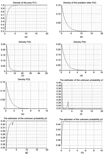
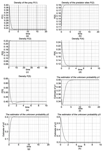
Clearly, the densities P

( )

2 to P

( )

5 in Figures 4(b)-(e) respectively, tend to the steady states. While, the density P

( )

1 in Figure 4(a) converges to the steady state. Also, the estimator p tˆ1

( )

in Figure 4(f) tends to the real value p1. While the

esti-mators pˆ2

( )

t and p tˆ3

( )

in Figure 4(g) and Figure 4(h) converge to the real values

2

p and p3 respectively. The steady state and the real values are represented by the

dotted lines.

The second numerical example of solution is given below.

[image:11.595.222.555.73.267.2]

(12)

[image:12.595.201.547.65.576.2]

Figure 4. The controlled densities and the estimators of the unknown parameters of the stochas-tic latstochas-tice gas of prey-predator model with pair approximation for some values of parameters and initial densities as follows:

1

k k2 k3 k4 k5 m1 m2 m3 p t1( ) p t2( ) p t3( )

1 0.45 0.3 1 1 5 5 5 0.22 0.35 0.45

1|0

P P2|0 P3|0 P4|0 P5|0 pˆ |1 0 pˆ |2 0 pˆ |3 0

(13)

[image:13.595.198.545.65.583.2]

Figure 5. The controlled densities and the estimators of the unknown parameters of the stochas-tic latstochas-tice gas of prey-predator model with pair approximation for some values of parameters and initial densities as follows:

1

k k2 k3 k4 k5 m1 m2 m3 p t1( ) p t2( ) p t3( )

2 5 3 2 1 1 2 2 0.4 0.4 0.2

1|0

P P2|0 P3|0 P4|0 P5|0 pˆ |1 0 pˆ |2 0 pˆ |3 0

(14)

[image:14.595.195.553.101.289.2]

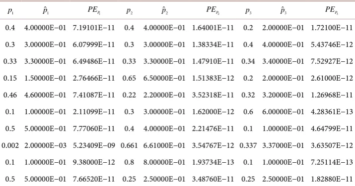
Table 2. The estimated values of the unknown parameters against the real values, and the per-centage errors for some real values.

1

p pˆ1 PEP1 p2 pˆ2 PEP2 p3 pˆ3 PEP3

0.4 4.00000E−01 7.19101E−11 0.4 4.00000E−01 1.64001E−11 0.2 2.00000E−01 1.72100E−11 0.3 3.00000E−01 6.07999E−11 0.3 3.00000E−01 1.38334E−11 0.4 4.00000E−01 5.43746E−12 0.33 3.30000E−01 6.49486E−11 0.33 3.30000E−01 1.47910E−11 0.34 3.40000E−01 7.52927E−12 0.15 1.50000E−01 2.76466E−11 0.65 6.50000E−01 1.51383E−12 0.2 2.00000E−01 2.61000E−12 0.46 4.60000E−01 7.41087E−11 0.22 2.20000E−01 3.52318E−11 0.32 3.20000E−01 1.26968E−11 0.1 1.00000E−01 2.11099E−11 0.3 3.00000E−01 1.62000E−12 0.6 6.00000E−01 4.28361E−13 0.5 5.00000E−01 7.77060E−11 0.4 4.00000E−01 2.21476E−11 0.1 1.00000E−01 4.64799E−11 0.002 2.00000E−03 5.23409E−09 0.661 6.61000E−01 3.54767E−12 0.337 3.37000E−01 3.63507E−12 0.1 1.00000E−01 9.38000E−12 0.8 8.00000E−01 1.93734E−13 0.1 1.00000E−01 7.25114E−13 0.5 5.00000E−01 7.66520E−11 0.25 2.50000E−01 3.48760E−11 0.25 2.50000E−01 1.82880E−11

( )

1

ˆ

p t and pˆ₂

( )

t in Figure 5(f) and Figure 5(g) tends to the real values p₁ and p2

respectively. While the estimator p tˆ3

( )

in Figure 5(h) converges to the real values

3

p . The steady states and the real values are represented by the dotted lines. The pre-vious figures show the approaching of the trajectories of the system to its steady states and approaching of the estimated values to the real values of the system unknown pa-rameters over time.

In the following, numerical calculation for the percentage error in each estimate for different real values of the system unknown parameters.

Table 2 represents the comparing between the real values of the unknown parame-ters and its estimated values, in addition to the infinitesimal values of the percentage errors indicate to a strong convergence between the assumed real values and its es-timated values so they are almost equally. These so good results are shown a high effi-ciency of the proposed Liapunov technique in the estimation process.

6. Conclusion

In this paper, we have introduced the mathematical model of stochastic lattice gas of prey-predator model with pair-approximation. The stability for this model has been discussed and it is found that this system has a chaos behavior. The estimators of the unknown parameters and the updating rules are derived according the conditions of the asymptotic stability. Some numerical solutions to show the stable system are pre-sented graphically.

References

[1] Dobrushin, R.L. (1971) Markov Processes with a Large Number of Locally Interacting Components: Existence of a Limit Process and Its Ergodicity. Problems of Information Transmission, 7, 149-164.

(15)

Reversible Cases and Some Generalization. Problems of Information Transmission, 7, 235- 241.

[3] El-Gohary, A. (2001) Optimal Control of the Genital Herpes Epidemic. Chaos, Solitons Fractals, 12, 1817-1822. http://dx.doi.org/10.1016/S0960-0779(00)00012-6

[4] El-Gohary, A. (2009) Chaos and Optimal Control of Equilibrium States of Tumor System with Drug. Chaos, Solitons and Fractals, 41, 425-435.

http://dx.doi.org/10.1016/j.chaos.2008.02.003

[5] El-Gohary, A. and Alwasel, I.A. (2009) The Chaos and Optimal Control of Cancer Model with Complete Unknown Parameters. Chaos, Solitons and Fractals, 42, 2865-2874. http://dx.doi.org/10.1016/j.chaos.2009.04.028

[6] Schinazi, R. (1997) Predatorprey and Host Parasite Spatial Stochastic Models. Annals of Applied Probability, 7, 1-9. http://dx.doi.org/10.1214/aoap/1034625250

[7] El-Gohary, A. and Al-Ruziza, A. (2003) Optimal Control of Non-Homogenous Prey Pre-dator Models During Finite and Infinite Time Intervals. Applied Mathematics and Com-putation, 146, 495-508. http://dx.doi.org/10.1016/S0096-3003(02)00601-X

[8] El-Gohary, A. and Al-Ruzaiza, A. (2007) Chaos and Adaptive Control in Two Prey, One Predator System with Nonlinear Feedback. Chaos, Solitons and Fractals, 34, 443-453. http://dx.doi.org/10.1016/j.chaos.2006.03.101

[9] El-Gohary, A. (2008) Chaos and Optimal Control of Cancer Self-Remission and Tumor System Steady States. Chaos, Solitons and Fractals, 37, 1305-1316.

http://dx.doi.org/10.1016/j.chaos.2006.10.060

[10] Al-Mahdi, A. and Khirallah, M. (2016) Bifurcation Analysis of a Model of Cancer. Euro-pean Scientific Journal, 12, 68-83.

[11] Khirallah, M. and Al-Mahdi, A. (2014) Stability Analysis of a Model of Cancer Treatment by Immunotherapy. European Journal of Scientific Research, 121, 161-173.

[12] Alwan, S. and El-Gohary, A. (2011) Chaos, Estimation and Optimal Control of Habitat De-struction Model with Uncertain Parameters. Computers and Mathematics with Applica-tions, 62, 4089-4099.

[13] El-Gohary, A. and Alwan, S. (2011) Estimation of Parameters and Optimal Control of the Genital Herpes Epidemic Model. Canadian Journal on Science and Engineering Mathemat-ics, 2, 31-41.

[14] Satulovsky, J. E and Tome, T. (1994) Stochastic Lattice Gas Model for a Predator-Prey Sys-tem. Physical Renew E, 49, 5073-5079.

[15] El-Gohary, A. and Alwan, S. (2011) Chaos and Optimal Control of Stochastic Lattice of Prey-Predator with Unknown Probabilities. International Journal of Mathematical Sciences and Applications, 1, 301-315.

[16] El-Gohary, A. (2005) Optimal Control of Stochastic Lattice of Prey-Predator Models. Ap-plied Mathematics and Computation, 160, 15-28.

(16)

Submit or recommend next manuscript to SCIRP and we will provide best service for you:

Accepting pre-submission inquiries through Email, Facebook, LinkedIn, Twitter, etc. A wide selection of journals (inclusive of 9 subjects, more than 200 journals)

Providing 24-hour high-quality service User-friendly online submission system Fair and swift peer-review system

Efficient typesetting and proofreading procedure

Display of the result of downloads and visits, as well as the number of cited articles Maximum dissemination of your research work

Submit your manuscript at: http://papersubmission.scirp.org/