Munich Personal RePEc Archive
Predicting bankruptcy using neural
networks and other classification
methods: the influence of variable
selection techniques on model accuracy
du Jardin, Philippe
Edhec Business School
2010
Online at
https://mpra.ub.uni-muenchen.de/44375/
Predicting bankruptcy using neural networks and other
classification methods: the influence of variable selection
techniques on model accuracy
Philippe du Jardin
EDHEC Business School, 393, promenade des Anglais, BP 3116, 06202 Nice Cedex 3, France
Abstract
We evaluate the prediction accuracy of models designed using different classification methods depending on the technique used to select variables, and we study the relationship between the structure of the models and their ability to correctly predict financial failure. We show that a neural network based model using a set of variables selected with a criterion that it is adapted to the network leads to better results than a set chosen with criteria used in the financial literature. We also show that the way in which a set of variables may represent the financial profiles of healthy companies plays a role in Type I error reduction.
Keywords: Financial failure, Variable selection, Neural network
1. Introduction
Since the early 1990’s, neural networks, and multi-layer perceptron neural networks in par-ticular, have been widely used to design bankruptcy prediction models [1]. These neural net-works make it possible to get around the statistical constraints of discriminant analysis, the main technique used to design such models since Altman [2]. In addition, their ability to represent non-linear relationships makes them well-suited to modeling the frequently non-linear relation-ship between the likelihood of bankruptcy and commonly used variables (i.e. financial ratios) [3].
Improving accuracy is certainly one of the most frequently addressed issues in bankruptcy prediction. The aim is to assess the conditions under which a model performs well. Some authors focused on identifying the methods of creating accurate models [2, 4, 5]. Others have studied the role of variables [6, 7] to assess whether some predictors are better than others (financial variables, ratios, non-financial variables). Still others have analyzed the types of failure a model is able to forecast. Indeed, traditional models are dichotomous and can classify only two groups. For this reason, a few authors have attempted to develop multi-state models, such as models to predict a final bankruptcy resolution (liquidation, reorganization, takeover) [8] or events that may affect the financial situation of a firm (non-payment of a debt, reduction of dividend payments)
[9]. Other authors have also analyzed the influence of sample size, group size, or the cost of mis-classification [10]. Only a very few have attempted to assess the contribution of variable selection techniques to the performance of a model [11, 12, 13]. To date, to our knowledge, nobody has done a comparative analysis of variable selection methods. Indeed, when the goal of the research is to find an effective means of improving prediction accuracy, whatever the modelling methods used to design models, one of the following strategies is used to choose explanatory variables: variables are selected because they are considered ”good” predictors in the financial literature, for their performance on univariate statistical tests (t test, F test, correlation test), or as a result of automatic search procedures using evaluation criteria tailored to discriminant analysis (Wilks’s lambda) or logistic regression (likelihood ratio). Only very few studies used other criteria. Table 1 illustrates the variable selection methods or criteria used by the main bankruptcy or financial failure studies that used a neural network. These criteria are rarely optimal when they are used in conjunction with a multi-layer perceptron neural network. When the aim of the research is to determine the conditions of replaceability of an existing model using new data or of a set a vari-ables optimized for a given method with another [14, 15], the choice is perhaps understandable. But when the aim is to study how to improve prediction accuracy, the methods used to select predictors are far from suitable for a non-linear method [16].
The aim of our research is therefore to analyze the influence of variable selection techniques on model accuracy, and particularly the fit of the evaluation criteria commonly used in the fi-nancial literature and a neural network, and to study the relationship that may exist between the structure of a model and its ability to correctly classify failing companies. The remainder of this paper is organized as follows. In Section 2, we present a literature review that explains our research questions. In Section 3, we describe the samples and methods used in our experiments. Finally, in Section 4, we present and discuss our results and, in Section 5, we summarize our main findings.
2. Literature review
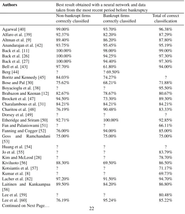
Table 1 presents the studies devoted to assessing the efficiency of classification or regression methods (neural networks, in particular), to designing bankruptcy or financial failure prediction systems, or to comparing the accuracy of various techniques, including neural networks, studies that attempt to identify the method best suited to designing prediction models. Table 1 also indicates methods or criteria used to select variables to be included in the models.
The main difficulty in choosing a set of predictors is the large number of variables that may be used. Indeed, the indicators most often chosen are based on financial ratios and then com-puted using balance sheets and income statements. There is almost no limit to designing financial ratios which indicate a given firm’s performance. We have analyzed nearly 200 scientific papers dealing with corporate failure prediction published in the last 50 years and found that more than 500 different ratios were used in the final models. It is for precisely this reason that variables are usually chosen from among those used in previous studies, that is, from among variables that have proven to be reliable failure predictors in the past. Indeed, often chosen are variables that were identified by the very first authors to assess the usefulness of financial ratios in pre-dicting corporate failure and by those who contributed to an understanding of the role played by multivariate statistical methods in the field of bankruptcy prediction, between the 1930’s and the 1970’s [2, 17, 18, 19, 20, 21, 22].
because the authors assume that a “good” model is made up of variables that demonstrate a good individual discrimination ability and low redundancy.
The final method of selecting predictors is to use an automatic search procedure to mine a large set of previously defined variables for the best subset(s), depending on a likewise pre-defined evaluation criterion. This procedure is usually a stepwise search alternating between backward and forward steps to explore the variable space; a Wilks’s lambda or a likelihood criterion is often used to evaluate the solutions.
Nevertheless, these three methods all have major drawbacks. The first method assumes that a variable that has proven to be a reliable indicator in a specific context will always be so in any other. All the experiments done to test the replicability of an existing model, to examine its per-formance with data not used during its design, show that the variables lose their initial properties when applied to other samples or used with methods other than those originally intended [23].
The second method assumes that a statistical test used to assess the individual discrimination ability of a variable is necessary for the design of a “good” model. However, a “good” model depends both on the interaction of the variables in a set, interaction that cannot be assessed through univariate tests, and on the way the variables fit the modelling method [24, 25], a fit that cannot be evaluated with such statistical tests.
Finally, the third method of selecting variables assumes that criteria optimized for discrim-inant analysis or logistic regression are suitable for other methods, and especially for neural networks. There is absolutely no reason to think that this assumption is valid. Moreover, Leray and Gallinari [16] have stated that since many parametric variable selection methods rely on the hypothesis that input-output variable dependence is linear or that input variable redundancy is well measured by the linear correlation of these variables, such methods are clearly ill-suited to non-linear methods, and hence to neural networks, since they are non-linear.
To overcome these limitations, some authors have explored other techniques such as genetic algorithms [11, 26, 27, 12, 28, 13, 29] or methods that fit a neural network [30, 31, 32, 33]. But these examples are very few and no comparative study has analyzed the influence of a variable selection technique on the predictive performance of a model. For this reason, this study intends to tackle this issue, in particular the influence of the evaluation criteria most often used with neural networks. To our knowledge, only one study [26] has compared a pair of sets of variables optimized for a discriminant analysis (stepwise method and F test), a logistic regression (stepwise method, Rao’s score test to add variables and a likelihood ratio test to discard variables) and a neural network (genetic algorithm), but this only to analyze the differences between the models in terms of accuracy over different prediction timeframes (one, two or three years).
of healthy companies.
3. Samples and methods
3.1. Samples and variables
Our experiments used data selected in 2006, and our results were computed in 2006 and 2007. We first selected French companies in the retail sector because in France, this sector traditionally accounts for the largest percentage of failed firms. Within this set of companies, we selected firms with an asset structure as homogenous as possible to control for the size effect and to allow comparisons of ratios. As there is no a priori rule for drawing a homogenous sample, we ran an Anova and a Mann-Whitney test on several breakdowns to find the most homogenous group, but also a group large enough to allow a relatively large sample size. These tests were computed on both failing and non-failing companies. Finally, the breakdown of companies into one group with assets of more thane750,000 and another with assets of less thane750,000 was the breakdown
in which the differences between the two groups, measured with all ratios, were the largest while allowing for a relatively large sample size. This is why we finally chose companies with assets of less thane750,000.
We then selected accounting data and computed only financial ratios. Data were collected within a single year, 2002, and we included just one variable (shareholder funds) from the pre-vious year 2001. When we selected healthy companies, we chose only companies in very good shape, that is, companies that were still in business in 2005. Moreover, we selected companies in operation for at least four years, because during the very first years of their lives, young, healthy companies often have a financial structure similar to that of failing companies. We also took into account the history of companies so as to select healthy firms that did not fail in the previous four years. Indeed, for several years after being reorganized, firms that went bankrupt and were then reorganized may reflect this bankruptcy in their financial statements and hence may look like failing companies.
Bankrupt companies were selected only if they were liquidated or reorganized in 2003, and at least 16 months after the publication of the annual report from 2002 so as to avoid any intentional distortion of financial statements.
We then try to design a well-balanced sample of young and old firms because young compa-nies usually have a much higher probability of bankruptcy than older ones. Finally, we selected bankrupt companies for which accounting data were available in 2002, and shareholder funds available in 2001, and for which bankruptcy was declared (liquidation or reorganization) by court decision in 2003.
This sample was used to estimate model accuracy. None of these companies used consolidated data.
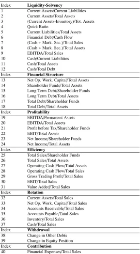
Finally we selected a set of 41 initial variables (Table 3) that can be broken up into seven categories that best describe company financial profiles: liquidity-solvency, financial structure, profitability, efficiency, turnover, withdrawal and contribution.
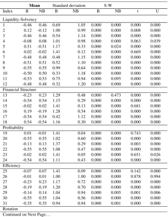
Table 4 shows the means and standard deviation of the distribution of each variable used to describe the discrepancy of the deviations that exist within and between the two groups of com-panies (figures computed using standardized data with 0 mean and unit variance). This table also indicates the results of a Shapiro-Wilks normality test and the results of two tests for differences between the means of each variable within each group. The normality test indicates that none of the variables are normally distributed at the conventional significance level of 5%. As a conse-quence, the non-parametric test (Mann-Whitney U test) is more reliable than the parametric one (Student t test). This test highlights that all variables except Total Sales/Total Assets, Current Assets/Total Sales and Labor Expenses/Total Sales, present significant differences between the two groups.
3.2. Modelling techniques
In the 200 papers dealing with financial failure prediction that we analyzed and that have been published since the late 1960’s, more than 50 classification or regression techniques are used. Three of these techniques predominate: discriminant analysis, logistic regression and multi-layer perceptron neural network. For this reason we selected these three methods.
All neural network parameters were defined a priori (topology, learning rate, momentum term, weight decay). To define these parameters, we used the following procedure. First, we randomly selected 50 sets of variables. Second, for each set of variables, we analyzed the results achieved with different values for each parameter: the learning rate varied from 0.1 to 0.5, with a step equal to 0.1, the momentum term from 0.5 to 0.9 (step= 0.1), the weight decay from 10−5 to 10−2 (step=10−1), and the number of hidden nodes from two to ten (step=1). We used only one hidden layer. Third, for each combination of parameters and each set of variables, we used a ten-cross validation technique to compute the error, and those that led to the lowest out-of-sample error calculated over the 50 sets were then selected for our experiments. We used data from 2002. Each of these 50 sets included on average 20 variables, with a minimum of 9 and a maximum of 27. It took roughly five days to compute all network parameters with 30 PCs running Windows, and an additional day to calculate and check the final results.
3.3. Variable selection methods
The variable selection methods we chose were those most commonly used with discriminant analysis, logistic regression and MLP.
First, we chose a technique that relies on a forward search procedure to explore a (sub) space of possible variable combinations, a Fisher F test to interrupt the search, and a Wilks’s lambda to compare variable subsets and determine the “best” one. This technique is especially optimized for discriminant analysis.
We then selected two other techniques optimized for logistic regression: a forward stepwise search and a backward stepwise search, with a likelihood statistic as an evaluation criterion of the solutions and aChi2 as a stopping criterion.
(filter methods) and one using the algorithm as an evaluation function (wrapper method). The first is a zero-order technique, Eq. (1), which uses the evaluation criteria designed by Yacoub and Bennani [34] and the second, Eq. (2), is a first-order method that uses the first derivatives of network parameters with respect to variables as an evaluation criterion. The last one relies on the evaluation of an out-of-sample error calculated with the neural network. We do not choose a second-order method, based on second derivatives of network parameters, in order to look into an equivalent number of points of comparison. With all these criteria, we use only a backward search procedure, rather than a forward or a sequential search, and the network is retrained after each variable removal.
The zero and first-order criterion were calculated as follows. With a network composed ofn
inputs, one hidden layer withhneurons and one output, wherewjiis the weight between input
iand neuron j in the hidden layer, and wj the weight between neuron j and the output, the
relevance or the saliencysof a variableimay be defined as:
Si= h
∑
j=1
(∑n|wji| k=1|Wjk|
·∑h|wj|
j′=1|wj′|
) (1)
Si=
1
N
N
∑
j=1
|∂yi
∂xji
| (2)
Wherexiis a variable,yis the output of the network calculated with only one neuron andN
the sample size.
To select variables, 1,000 random bootstrap samples were drawn with replacement from the dataset of year 2002 (500 companies). Each bootstrap sample included 500 companies. We used the following three-step procedure to select variables:
• During the first step, each selection method was used to select variables with these 1,000 bootstrap samples.
• Then, to identify important variables, those that were included in more than 70% of the selection results were selected. But this procedure might lead to remove highly correlated variables. Indeed, if two variables are correlated, the selection results may contain one or the other of these two variables while none of them will be included in 70% of the results. To avoid discarding potentially relevant but highly correlated variables, we used a second step. During the second step, variable pairs in which one or both variables were included in more than 90% of the bootstrap selections were considered pairs containing a relevant variable. Then, for each identified pair, the variable that occurs in most of the selection results was chosen.
• Finally, during the third step, variables that were selected during the first and second step were used to choose the final subsets. To choose these final subsets, the process used during the first step was repeated once.
3.4. Model development
• During the first step, the sample of year 2002 was randomly divided into two sub-samples: a learning sampleAof 450 companies and a validation sampleVof 50 companies.
• During the second step, twenty-five bootstrap samples were drawn with replacement from A, each bootstrap sample included 450 companies and, for each selected set of variables, used to estimate as many models as bootstrap samples.
• Finally, during the third step, the resulting models were used to classify the observations of sampleVthanks to a majority voting scheme. The cut-offpoint for classifying a firm as healthy or bankrupt was set as that which maximizes the overall rate of correct clas-sifications. These three steps were repeated 100 times and the out-of-sample error was first estimated, along with a validation sample, and then re-estimated using the 25×100 models, along with a test sample of 520 companies.
• We used such a procedure to reduce the variance of prediction error caused by data insta-bility. Indeed, financial ratios are always far from being normally distributed and contain many outliers. As a consequence, a small change in the data may produce a substan-tial change in the results. It is for this reason that we have chosen this bootstrap scheme [35, 36].
Moreover, the figures used to implement the bootstrap scheme (proportion of companies belonging to the learning sample and test sample, number of replicates of the procedure) were inspired by those used by Breiman [35] for a similar procedure. The computational time required to achieve the development of all models was quite large as it took several weeks, using 30 PCs running Windows.
4. Results and discussion
4.1. Selected variables
Tables 5, 6 and 7 show the six sets of variables that appeared in the selection results. Those that were chosen in more than 70% of the results were included in the final models. Each variable name is followed by its frequency of selection.
4.2. Selected variables and individual discrimination power
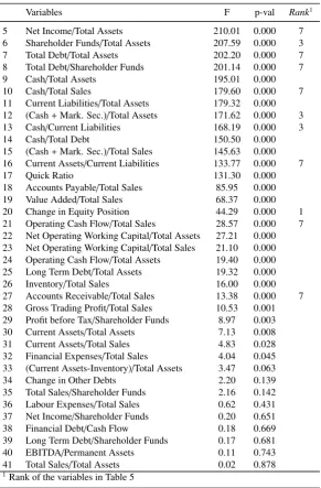
contrast, variables with high discrimination ability, such as EBITDA/Total Sales, Cash/Total As-sets, Current Liabilities/Total Assets, or Cash/Total Debt, are not selected with any selection techniques.
As a consequence, it appears that using a t or an F test for a selection or pre-selection of the inputs of a neural network is unreliable as these tests may lead to the choice of unnecessary variables as well as to the removal of variables of great interest. This might well have been the case here, with the Change in Equity Position, for which the F test is quite low even though this variable is in fact relevant according to the neural network. Indeed, selection with a Wilks’s lambda removes this variable. But when the value of an F test falls below a certain level, the only other variable selected is Accounts Receivable/Total Sales (which is selected only once).
4.3. Model accuracy
We then analyzed the relationship between modelling techniques and variable selection meth-ods. The aim was to ascertain whether any pairs perform better than others and to study the be-havior of a neural network while using sets of variables that were optimized for other methods.
We first measured the accuracy of “modelling method/selection technique” combinations, but only for those for which the evaluation criterion suited the classification technique. We compared the results of the following six pairs of methods: discriminant analysis-Wilks’s lambda, logis-tic regression-likelihood criterion (with two search procedures), and neural network-zero-order, first-order, and error criteria. As Tables 11 and 12 show, the neural network outperforms dis-criminant analysis and to a lesser extent logistic regression. Indeed, the best result−93.85%−is achieved with a neural network on the test samples, followed by that for logistic regression with 90.77% and discriminant analysis with 85.19%. We then analyzed the results obtained when a modelling technique is used with a selection procedure for which the fit is not deemed accept-able. The results were computed on the validation samples. Table 13 shows the results obtained with the set of variables selected with a Wilks’s lambda and those selected with a likelihood criterion. Table 14 shows the results calculated with the three sets of variables optimized for a neural network
Table 13 shows that variable selection based on a variance criterion (i.e., Wilks’s lambda) leads to poor results; the adequate classification rate of 87.20% achieved with discriminant anal-ysis is slightly lower with the other two methods. The criterion used here relies on assumptions that dovetail with those on which discriminant analysis is founded. It is not surprising that vari-ables that cannot satisfactorily classify a high percentage of firms with discriminant analysis are unable to provide good results with other methods; the models built with logistic regression and the neural network lead to very similar results. Therefore, this criterion is clearly ill-suited to non-linear techniques.
cor-rect classification of 93.59%, 88.01% and 83.60%. However, with a first-order criterion there is a decrease, with figures of 92.82%, 89.19% and 84.45%.
Thus, we can see that, the neural network leads to far better results than other methods, especially with an error criterion, which is not really surprising since this criterion is both the evaluation criterion of the variable relevance and the measure of this relevance. This is a very characteristic feature of wrappers because the inductive algorithm is used directly during variable selection. This result is consistent with what we might expect. The zero-order criterion’s outper-formance of a first-order criterion can be put down primarily to chance as there is no evidence that the former is better than the latter.
Neural models, when developed with appropriate variables, are thus much more reliable than logistic or discriminant models. Nevertheless, logistic models seem to better fit the data than discriminant models, whatever the variables used. In addition, with an error criterion, a logistic model produces 90.00% accuracy, whereas the neural model achieves 94.03%, leaving the logistic model−at 84.38%−far behind.
The accuracy of a model is in part the result of the intrinsic characteristics of the modelling technique and in part that of the fit of this technique and the variable selection procedure in-volved in its design. In bankruptcy prediction, all the experiments that have been done with large samples show that both financial ratios and a probability of bankruptcy behave in a non-linear manner. It is precisely for this reason that, as long as this non-linearity cannot be taken into ac-count, it is hard to develop accurate models. Although using a selection criterion that fits logistic regression to design a neural model may be relevant, the choice of a criterion that fits discrimi-nant analysis for the same purpose should not be recommended. It is necessary, at the very least, to consider other solutions.
4.4. Relationship between the structure of the models and their ability to correctly classify failing companies
As stated in the literature review, financial failure prediction models lead to better results when they predict that a company will remain healthy in the future as opposed to when they predict that it will fail. We can observe the same results with discriminant analysis (Table 11) and, to a lesser extent, with logistic regression. It appears that sound companies have a much wider variety of financial profiles than failing companies, with some of them having profiles similar to those of failing companies. Failing firms may continue to do business, but it is much more unusual for healthy firms to go suddenly bankrupt. This suggests there are sub-groups of sound companies whose financial profiles are so similar to those of failing companies that they move the boundary between the two groups in such a way that the models tend to identify bankrupt firms as healthy, and as a consequence lead to weaker results when classifying bankrupt firms.
To study this issue, we have used a Kohonen map to analyze the profiles of each group of firms and data from 2002. To determine the form of the map (i.e., the number of rows and columns), we first used Sammon’s mapping method to examine the topology of the data. This map provides a general overview of the shape of the data and makes it possible to determine whether we may use a rectangular or square map. We have chosen a square map as there was no evidence that a rectangular one was better; it is made up of 100 neurons, 10 per line and 10 per column, one-fifth of the year 2002 sample.
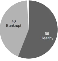
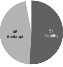
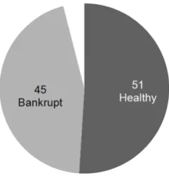
sure that, using Sammon’s mapping method, no significant folding or stretching was visible on the map at the end of the learning phase. We first analyzed the distribution of the neurons by group of companies, whether they represent sound or unsound firms. Each map was designed using one of the six sets of variables we selected. Figures 1 to 6 show the number of neurons for each class in each each map (one map per set of variables). The dark grey part of the figures represents healthy companies, the light grey, bankrupt companies, and the white corresponds to neither. To assign a neuron to a class, we used a majority voting scheme, depending on the class of the nearest observations to a neuron.
The characteristics of the map are shown in Table 15. For each map (i.e., each set of vari-ables), Table 15 presents the number of neurons in each group, the number of variables, the quantization error, that is, the information loss because of the projection of the input space onto a plan, the standard deviation of this error and the p-value of a Student t test for differences between the quantization error of the two groups. The error corresponds to the mean of the Euclidean dis-tances computed between the neurons belonging to the same class and the firms that were the closest to these neurons. In Table 15, we can see that each group is represented by a somewhat different number of neurons. On average, healthy companies are coded using 52 neurons, com-pared with 45 neurons for bankrupt companies. The tiniest difference, which appears twice, can be observed with the set of variables selected using a Wilks’s lambda and the set selected using a first-order criterion, where healthy firms are coded with 50 neurons and bankrupt firms with 49. The largest difference is due to the set of variables chosen on the basis of the error criterion, where healthy companies are coded with 56 neurons and bankrupt companies with 40. This find-ing reinforces the idea we mentioned in our look at the results of many bankruptcy prediction models published in the financial literature. Indeed, in this literature healthy firms are more often correctly classified than failing firms, as if the financial profiles of the former were much more complex and multiform than the profiles of the latter. As a consequence, the profiles of some healthy companies seem to be similar to the profiles of failing companies. Using a Kohonen map and financial ratios to develop a typology of companies, P´erez [37] noted that healthy firms would present a much wider spectrum of profiles than failing firms, without further analysis.
We can also notice in Table 15 that the quantization error associated with bankrupt compa-nies is larger than the one associated with healthy compacompa-nies, and the difference is statistically significant at the threshold of 5% in three cases out of six, and nearly significant in a fourth one if we consider the first-order criterion. This error is partly due to the difference between the number of neurons in each class when this difference exists. Once a group is quantified by a number of prototypes lower than another one, we may consider that the quality of its quantization is less than the quality of the other. This is probably the case in our experiments. However another fac-tor may have an influence when the number of neurons in each group is similar. We used facfac-tor analysis in order to design sub-groups in each class (healthy vs bankrupt) and we found that the difference we can observe in the quantization error between healthy and bankrupt companies is also partly due to a few sub-groups of bankrupt companies (which are much heterogenous than the others). However, on average, healthy companies present a wider variety of financial profiles than bankrupt firms.
Table 17 that there is a relationship between the ability to classify failing firms correctly and the structure of the maps. Indeed, the models that achieve much higher correct classification rates for healthy firms than for bankrupt firms are designed on profiles where healthy companies can express all their diversity. As a result, the corresponding maps are based on a slightly different number of neurons encoding each class. The first three lines in Table 17−two of three models are far better at identifying failed firms than at identifying healthy ones−summarize the situation well. At the bottom of Table 17, we find models that achieve similar or less good results when classifying healthy companies, for which the underlying profiles are encoded using roughly the same number of neurons.
However, these results should be considered with caution since they rely on a single sample, and they only express a trend. Indeed, the relationship we have just analyzed is not true in all cases. Our results should therefore be confirmed by further studies, and if they are confirmed, they would make it possible to show that some financial profiles (i.e., sets of ratios) may intrinsi-cally better discriminate between failing firms and sound firms than do others. For the moment, one of the main techniques used to improve the classification rate of failing firms is to look for an optimal cut-offpoint that will be able to maximize this rate while keeping the broader classifi-cation rate in a suitable range. Therefore, it will be valuable if some variables result in improved classification of failing firms; the advantage of this improvement is that it would make possible a simplified calculation to take into account the asymmetry of the costs of mistaken identification of failing and healthy companies.
5. Conclusion
We have shown that there is a relationship between the discrimination ability of a variable, as measured with a t test or an F test, and its susceptibility to selection by an automatic procedure that relies on other measures, but we have also found a discrepancy in this relationship which indicates that such statistical tests should not be used alone if the purpose of the selection is to create a neural model. As a consequence, we may use them-but with extreme caution-to build non-linear models, and if we intend to do so, we would do well to use them in conjunction with other techniques. However, even if criteria that fit neural networks lead to accurate classification results, in practice, it is hard to choose the right criterion. Indeed, the performance of a criterion depends on data structure. For instance, Leray and Gallinari [16] have demonstrated that the accuracy of a model designed with a specific criterion strongly depends on the level of correlation between variables, the degree of linear separability of data and the level of noise. These results clearly indicate the drawbacks of an approach based only on a single selection criterion, even is this criterion is well-suited to the modelling techniques used.
[1] A. Atiya, Bankruptcy prediction for credit risk using neural networks: a survey and new results, IEEE Transactions on Neural Networks 7 (2001) 929–935.
[2] E. Altman, Financial ratios, discriminant analysis and the prediction of corporate bankruptcy, Journal of Finance 19 (1968) 589–609.
[3] E. Laitinen, T. Laitinen, Bankruptcy prediction: application of the taylor’s expansion in logistic regression, Inter-national Review of Financial Analysis 9 (2000) 327–349.
[4] M. Odom, R. Sharda, A neural network model for bankruptcy prediction, in: the IEEE International Joint Confer-ence on Neural Networks, 1990, pp. 163–168.
[5] J. Ohlson, Financial ratios and the probabilistic prediction of bankruptcy, Journal of Accounting Research 18 (1980) 109–131.
[6] K. Keasey, R. Watson, Non-financial symptoms and the prediction of small company failure: a test of argenti’s hypothesis, Journal of Business Finance and Accounting 14 (1987) 335–354.
[7] C. Mossman, G. Bell, L. Swartz, H. Turtle, An empirical comparison of bankruptcy models, Financial Review 33 (1998) 35–53.
[8] N. Kumar, R. Krovi, B. Rajagopalan, Financial decision support with hybrid genetic and neural based modeling tools, European Journal of Operational Research 103 (1997) 339–349.
[9] E. Altman, G. Marco, F. Varetto, Corporate distress diagnosis: comparisons using linear discriminant analysis and neural network - the italian experience, Journal of Banking and Finance 18 (1994) 505–529.
[10] G. Karels, A. Prakash, Multivariate normality and forecasting of business bankruptcy, Journal of Business Finance and Accounting 14 (1987) 573–593.
[11] B. Back, G. Oosterom, K. Sere, M. van Wezel, A comparative study of neural networks in bankruptcy prediction, in: the 10th Conference on Artificial Intelligence Research in Finland, 1994, pp. 140–148.
[12] A. Brabazon, P. Keenan, A hybrid genetic model for the prediction of corporate failure, Computational Management Science 1 (2004) 293–310.
[13] R. Sexton, R. Sriram, H. Etheridge, Improving decision effectiveness of artificial neural networks: a modified genetic algorithm approach, Decision Sciences 34 (2003) 421–442.
[14] P. Coats, L. Fant, Recognizing financial distress patterns using a neural network tool, Financial Management 22 (1993) 142–154.
[15] E. Rahimian, S. Singh, T. Thammachote, R. Virmani, Bankruptcy prediction by neural networks, in: Neural Net-works in Finance and Investing: Using Artificial Intelligence to Improve Real-World Performance, 1993, pp. 159– 171.
[16] P. Leray, P. Gallinari, Feature selection with neural networks, Behaviormetrika 26 (1998) 145–166.
[17] E. Altman, R. Haldeman, P. Narayanan, Zeta analysis: a new model to identify bankruptcy risk of corporations, Journal of Banking and Finance 1 (1977) 29–51.
[18] W. Beaver, Financial ratios as predictors of failure, empirical research in accounting, selected studies, Journal of Accounting Research 4 (1996) 71–111.
[19] M. Blum, Failing company discriminant analysis, Journal of Accounting Research 12 (1974) 503–512.
[20] E. Deakin, A discriminant analysis of predictors of business failures, Journal of Accounting Research 10 (1972) 167–179.
[21] C. Merwin, Financing small corporations in five manufacturing industries, in: National Bureau of Economic Re-search, Financial Research Program III, Studies in Business Financing, 1942, pp. 1926–1936.
[22] J. Ramser, L. Foster, A demonstration of ratio analysis, in: Bulletin n 40, University of Illinois, Bureau of Business Research, 1931.
[23] H. Ooghe, H. Claus, N. Sierens, J. Camerlynck, International comparison of failure prediction models from different countries: an empirical analysis, in: Working Paper, Ghent University, 1999.
[24] G. John, R. Kohavi, K. Pfleger, Irrelevant features and the subset selection problem, in: the 11th International Conference, 1994, pp. 121–129.
[25] R. Kohavi, A study of cross validation and bootstrap for accuracy estimation and model selection, in: the 14th International Joint Conference on Artificial Intelligence, 1995, pp. 1137–1143.
[26] B. Back, G. Oosterom, K. Sere, M. van Wezel, Choosing bankruptcy predictors using discriminant analysis, logit analysis and genetic algorithms, in: Technical Report, Turku Centre for Computer Science, 1996.
[27] B. Back, G. Oosterom, K. Sere, Neural networks and genetic algorithms for bankruptcy predictions, Expert Systems with Applications 11 (1996) 407–413.
[28] C. Kim, R. McLeod, Expert, linear models and nonlinear models of expert decision making in bankruptcy predic-tion: a lens model analysis, Journal of Management Information Systems 16 (1999) 189–206.
[29] J. Wallrafen, P. Protzel, H. Popp, Genetically optimized neural network classifiers for bankruptcy prediction - an empirical study, in: the 29th Hawaii International Conference on System Sciences, 1996, pp. 419–426.
[31] C. Charalambous, A. Charitou, F. Kaourou, Application of feature extractive algorithm to bankruptcy prediction, in: the IEEE-INNS-ENNS International Joint Conference on Neural Networks, 2000, pp. 303–308.
[32] T. Sen, P. Ghandforoush, C. T. Stivason, Improving prediction of neural networks: a study of two financial predic-tion tasks, Journal of Applied Mathematics and Decision Sciences 8 (2004) 219–233.
[33] E. Tyree, J. Long, Bankruptcy prediction models: probabilistic neural networks versus discriminant analysis and backpropagation neural networks, in: Working Paper, Department of Business Computing, City University, 1996. [34] M. Yacoub, Y. Bennani, Hvs: a heuristic for variable selection in multilayer artificial neural network classifier, in:
the International Conference on Artificial Neural Networks and Intelligent Engineering, 1997, pp. 527–532. [35] L. Breiman, Bagging predictors, Machine Learning 24 (1996) 123–140.
[36] Y. Grandvalet, Bagging equalizes influence, Machine Learning 55 (2004) 251–270.
[37] M. P´erez, De l’analyse de la performance `ala pr´evision de d´efaillance: les apports de la classification neuronale, in: PhD Dissertation, Jean-Moulin University, Lyon III, 2002.
[38] M. Boyacioglu, Y. Kara, O. Baykan, Predicting bank financial failures using neural networks, support vector ma-chines and multivariate statistical methods: a comparative analysis in the sample of savings deposit insurance fund (sdif) transferred banks in turkey, Expert Systems with Applications 36 (2009) 3355–3366.
[39] E. Alfaro, N. Garcia, M. Games, D. Ellison, Bankruptcy forecasting: an empirical comparison of adaboost and neural networks, Decision Support Systems 45 (2008) 110–122.
[40] A. Agarwal, Abductive networks for two-group classification: a comparison with neural networks, ESANN 2008, European Symposium on Artificial Neural Networks, Bruges, Belgium 15 (1999) 1–12.
[41] R. L. Wilson, R. Sharda, Bankruptcy prediction using neural networks, Decision Support System 32 (1994) 545– 557.
[42] M. Anandarajan, P. Lee, A. Anandarajan, Bankruptcy prediction of financially stressed firms: an examination of the predictive accuracy of artificial neural networks, international journal of intelligent systems in accounting, Finance and Management 10 (2001) 69–81.
[43] T. Bell, G. Ribar, J. Verchio, Neural nets vs. logistic regression: a comparison of each model’s ability to pre-dict commercial bank failures, in: the 1990 Deloitte and Touche-University of Kansas Symposium on Auditing Problems, 1990, pp. 29–58.
[44] D. Berg, Bankruptcy prediction by generalized additive models, in: Statistical Report, University of Oslo, Depart-ment of Mathematics, 2005.
[45] J. Boritz, D. Kennedy, Effectiveness of neural network types for prediction of business failure, Expert Systems with Applications 9 (1995) 589–609.
[46] T. Sen, P. Ghandforoush, C. T. Stivason, Feedforward neural networks in the classification of financial information, European Journal of Finance 3 (1997) 183–202.
[47] P. Brockett, W. Cooper, L. Golden, U. Pitakgong, A neural network method for obtaining an early warning of insurer insolvency, Journal of Risk and Insurance 61 (1994) 402–424.
[48] A. Charitou, E. Neophytou, C. Charalambous, Predicting corporate failure: empirical evidence for the uk, European Accounting Review 13 (2004) 465–497.
[49] D. R.E., R. Edmister, J. Johnson, Bankruptcy prediction using artificial neural systems, in: Working Paper, Univer-sity of Mississippi, School of Business, 1995.
[50] H. Etheridge, R. Sriram, A comparison of the relative costs of financial distress models: artificial neural networks, logit and multivariate discriminant analysis, International Journal of Intelligent Systems in Accounting, Finance and Management 6 (1997) 235–248.
[51] A. Fan, M. Palaniswami, Selecting bankruptcy predictors using a support vector machine approach, in: the IEEE-INNS-ENNS International Joint Conference on Neural Networks, 2000, pp. 354–359.
[52] K. Fanning, K. Cogger, A comparative analysis of artificial neural networks using financial distress prediction, International Journal of Intelligent Systems in Accounting, Finance and Management 3 (1994) 241–252. [53] E. Goss, H. Ramchandani, Comparing classification accuracy of neural networks, binary logit regression and
dis-criminant analysis for insolvency prediction of life insurer, Journal of Economics and Finance 19 (1995) 1–18. [54] C. Huang, R. Dorsey, M. Boose, Life insurer financial distress prediction: a neural network model, Journal of
Insurance Regulation 13 (1994) 131–167.
[55] I. H. H. Jo, H. Lee, Bankruptcy prediction using case-based reasoning, neural networks and discriminant analysis, Expert Systems with Applications 13 (1997) 97–108.
[56] K. Kiviluoto, Predicting bankruptcies with the self-organizing map, Neurocomputing 21 (1998) 191–220. [57] S. Kotsiantis, D. Tzelepis, E. Koumanakos, V. Tampakas, Efficiency of machine learning techniques in bankruptcy
prediction, in: 2nd International Conference on Enterprise Systems and Accounting, 2005, pp. 39–49.
[58] T. Laitinen, M. Kankaanpaa, Comparative analysis of failure prediction methods: the finnish case, European Ac-counting Review 8 (1999) 67–92.
[60] K. Lee, D. Booth, P. Alam, A comparison of supervised and unsupervised neural networks in predicting bankruptcy of korean firms, Expert Systems with Applications 29 (2005) 1–16.
[61] M. Leshno, Y. Spector, Neural network prediction analysis: the bankruptcy case, Neurocomputing 10 (1996) 125– 147.
[62] X. Li, J. Gupta, Neural networks in financial failure prediction: a revisit, in: the Annual Decision Sciences Institute Conference, 2002, pp. 233–238.
[63] T. McKee, M. Greenstein, Predicting bankruptcy using recursive partitioning and a realistically proportioned data set, Journal of Forecasting 19 (2000) 219–230.
[64] S. Min, J. Lee, I. Han, Hybrid genetic algorithms and support vector machines for bankruptcy prediction, Expert Systems with Applications 31 (2006) 652–660.
[65] J. Min, Y. Lee, Business failure prediction with support vector machines and neural networks: a comparative study, in: the 9th Asia-Pacific Decision Sciences Institute Conference, 2004.
[66] J. Min, Y. C. Lee, Bankruptcy prediction using support vector machine with optimal choice of kernel function parameters, Expert Systems with Applications 28 (2005) 603–614.
[67] P. Pendharkar, A threshold-varying artificial neural network approach for classification and its application to bankruptcy prediction problem, Computers and Operations Research 32 (2005) 2561–2582.
[68] S. Piramuthu, H. Ravagan, M. J. Show, Using feature construction to improve the performance of neural networks, Management Science 44 (1998) 416–430.
[69] P. Pompe, A. Feelders, Using machine learning, neural networks and statistics to predict corporate bankruptcy, Microcomputers in Civil Engineering 12 (1997) 267–276.
[70] L. Salchenberger, E. Cinar, N. Lash, Neural networks: a new tool for predicting thrift failures, Decision Sciences 23 (1992) 899–916.
[71] S. Shin, Y. Lee, A genetic algorithm application in bankruptcy prediction modeling, Expert Systems with Applica-tions 23 (2003) 321–328.
[72] K. Tam, M. Kiang, Managerial applications of neural networks: The case of bank failure predictions, Management Science 38 (1992) 926–947.
[73] C. Tan, H. Dihardjo, A study on using artificial neural networks to develop an early warning predictor for credit union financial distress with comparison to the probit model, Managerial Finance 27 (2001) 56–77.
[74] W. Tung, C. Quek, P. Cheng, Genso-ews: a novel neural-fuzzy based early warning system for predicting bank failures, Neural Networks 17 (2004) 567–587.
[75] A. Vieira, P. Castillo, J. Merelo, Application of hlvq and g-prop neural networks to the problem of bankruptcy prediction, in: Application of HLVQ and G-Prop neural networks to the problem of bankruptcy prediction, 2003, pp. 655–652.
[76] D. West, S. Dellana, J. Qian, Neural network ensemble strategies for financial decision application, Computers and Operations Research 32 (2005) 2543–2559.
[77] C. Wu, G. Tzeng, Y. Goo, W. Fang, A real-valued genetic algorithm to optimize the parameters of support vector machine for predicting bankruptcy, Expert Systems with Applications 32 (2007) 397–408.
[78] Z. Yang, R. G. Harrison, Analysing company performance using templates, Intelligent Data Analysis 6 (2002) 3–15.
[79] Z. R. Yang, M. B. Platt, H. D. Platt, Probabilistic neural networks in bankruptcy prediction, Journal of Business Research 44 (1999) 67–74.
[80] J. Yim, H. Mitchell, A comparison of corporate failure models in australia: hybrid neural networks, logit models and discriminant analysis, in: Working Paper, RMIT Business, School of Economics and Finance, 2002. [81] J. Yim, H. Mitchell, A comparison of corporate distress prediction models in brazil: hybrid neural networks,
logit models and discriminant analysis, in: Working Paper, Universidade Federal de Minas Gerais, Economics Department, Nova Economia, 2005.
[82] R. Lacher, P. Coats, S. Sharma, L. Fant, A neural network for classifying the financial health of a firm, European Journal of Operational Research 85 (1995) 53–65.
6. Figures
Figure 1: Number of neurons in the Kohonen map per class. Set of variables selected using a Wilks’s lambda criterion and a stepwise search
[image:18.595.236.360.395.525.2]Figure 3: Number of neurons in the Kohonen map per class. Set of variables selected using a likelihood criterion and a forward stepwise search
[image:19.595.236.360.483.617.2]Figure 5: Number of neurons in the Kohonen map per class. Set of variables selected using a zero order criterion and a backward search
7. Tables
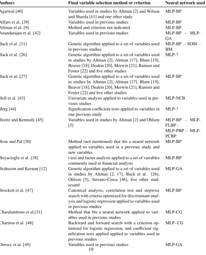
Table 1: Variable selection methods used in major studies which aimed to design bankruptcy prediction models with neural network models
Authors Final variable selection method or criterion Neural network used
Agarwal [40] Variables used in studies by Altman [2] and Wilson
and Sharda [41] and one other study
MLP-BP
Alfaro et al. [39] Variables used in previous studies MLP-BP
Altman et al. [9] Method and criterion not indicated MLP-BP
Anandarajan et al. [42] Variables used in previous studies BP -
MLP-GA Back et al. [11] Genetic algorithm applied to a set of variables used
in previous studies
MLPBP SOM -BM
Back et al. [26] Genetic algorithm applied to a set of variables used in studies by Altman [2], Altman [17], Blum [19], Beaver [18], Deakin [20], Merwin [21], Ramser and Foster [22] and five other studies
MLP-?
Back et al. [27] Genetic algorithm applied to a set of variables used in studies by Altman [2], Altman [17], Blum [19], Beaver [18], Deakin [20], Merwin [21], Ramser and Foster [22] and five other studies
MLP-BP
Bell et al. [43] Univariate analysis applied to variables used in pre-vious studies
MLP-NCB
Berg [44] Signification coefficient tests applied to variables in one previous study
MLP-?
Boritz and Kennedy [45] Variables used in studies by Altman [2] and Ohlson [5]
BP - MLPFLBP
-PBP - MLP-PCBP
Bose and Pal [30] Method (not mentioned) that fits a neural network applied to variables used in a previous study and new variables
MLP-BP
Boyacioglu et al. [38] t test and factor analysis applied to a set of variables commonly used in financial analysis
MLP-BP
Brabazon and Keenan [12] Genetic algorithm applied to a set of variables used in studies by Altman [2, 17], Back et al. [26], Ohlson [5], Serrano-Cinca [46], five other stud-iesand
MLP-GA
Brockett et al. [47] Canonical analysis, correlation test and stepwise search with criteria optimized for discriminant anal-ysis and logistic regression applied to variables used in previous studies
MLP-BP
Charalambous et al.[31] Method that fits a neural network applied to vari-ables used in previous studies
MLP-CG
Charitou et al. [48] Backward and forward search with a criterion op-timized for logistic regression, and coefficient sig-nification tests applied applied to variables used in previous studies
MLP- CG
Etheridge and Sriram [50] Not mentioned SOM - PNN Fan and Palaniswami [51] Distance measure between the centroid of the
groups applied to variables used in studies by Alt-man [2], Ohlson [56], and one other study, and vari-ables commonly used in financial literature
MLP-BP - LVQ
Fanning and Cogger [52] Variables used in one previous study MLP-BP - GANN
Goss and Ramchandani [53] Variables used in one previous study MLP-BP
Huang et al. [54] Variables used by insurance company regulation au-thority
MLP-GA
Jo et al. [55] t test applied to variables used in studies by Beaver [18], Altman [2], Blum [40], Deakin [20], Odom and Sharda [4], Ohlson [5], and fourteen other stud-ies
MLP-BP
Kim and McLeod [28] Judgment of an expert applied to variables com-puted with a factor analysis and other variables commonly used in the financial literature
MLP-GA
Kiviluoto [56] Not mentioned SOM - SOM-RBF
Kotsiantis et al. [57] Relief method applied to a set of variables com-monly used in the literature
MLP-RBF
Kumar et al. [8] Stepwise search with a criterion optimized for dis-criminant analysis applied to variables used by Alt-man [2] and in two other studies
MLP-BP
Lacher et al. [41] Variables used in study by Altman [2] CasCor
Laitinen and Kankaanpaa [58] Variables used in previous studies MLP-BP
Lee et al. [59] Stepwise search with a criterion optimized for dis-criminant analysis applied to variables used in pre-vious studies
MLP-BP - SOM-MLP
Lee et al. [60] Variables used in study by Altman [2] MLP-LM - SOM
Leshno and Spector [61] Judgment and correlation test applied to variables used in previous studies and variables used in study by Altman [2]
MLP-BP - MLP-?
Li and Gupta [62] Variables used in one previous study MLP-GA
McKee and Greenstein [63] Variables used in one previous study ?
Min et al. [64] Stepwise search with criteria optimized for discrim-inant analysis and logistic regression, and t test ap-plied to variables used in previous studies
?
Min and Lee [65] Stepwise search with criteria optimized for discrim-inant analysis logistic regression, and t test and
MLP-BP
Min and Lee [66] Factor analysis, t tests and stepwise search with cri-teria optimized for discriminant analysis and logis-tic regression
MLP-BP
Odom and Sharda [4] Variables used in study by Altman [2] MLP-BP
Pendharkar [67] Variables used in studies by Altman [2] and Altman et al. [17]
BP - MLP-GA
Piramuthu et al. [68] Classification tree and symbolic rules MLP-BP
Pompe and Feelders [69] Judgment of an expert applied to financial variables commonly used by financial experts to predict cor-porate failure
MLP-BP
Salchenberger et al. [70] Multiple regression applied to variables commonly used in financial analysis
MLP-BP
Serrano-Cinca [46] Variables used in one previous study MLP-BP Sexton et al. [13] Genetic algorithm applied to variables commonly
used in financial analysis
MLP-GA
Shin et Lee [71] Stepwise search with a criterion optimized for dis-criminant analysis and t test
MLP-BP
Tam and Kiang [72] Variables that belong to the following financial cat-egories: asset, income, liquidity
MLP-BP
Tan and Dihardjo [73] Variables used in two previous studies MLP-BP
Tung et al. [74] Correlation test applied to variables used in previ-ous studies
MLP-BP
-GSOFNN Tyree and Long [33] Method that fits a neural network (sensitivity
mea-sure) and stepwise search with a criterion optimized for discriminant analysis
MLP-BP - PNN
Vieira et al. [75] Variables used in previous studies HLVQ - G-Prop
Wallrafen et al. [74] Genetic algorithm applied to variables that belong to the following financial categories: liquidity, prof-itability, asset, solidity, debt and reimbursement ability
MLP-GA
West et al. [76] Variables used in study by Altman [2] MLP-BP
Wilson and Sharda [41] Variables used in study by Altman [2] MLP-BP
Wu et al. [77] Variables used in previous studies MLP-BP
Yang and Harrison [78] Stepwise search with a criterion optimized for dis-criminant analysis applied to variables commonly used in financial analysis
MLPBP PNN -RHPNN
Yang et al. [79] Variables used in one previous study MLP-BP - PNN
Yim and Mitchell [80] Variables used in previous studies MLP-BP
Yim and Mitchell [81] Variables that belong to the following financial cat-egories: liquidity, profitability, structure, asset
MLP-BP
This table indicates, in addition to the variable selection methods or criteria that were used, the name of the neural network and the name of the algorithm used during the learning process. For example, MLP-BP corresponds to a multi-layer perceptron neural network trained using a back-propagation method. This learning algorithm is used in more than 75% of the research works mentioned here, whereas the MLP is used in almost all experiments. The acronyms are those used by the authors. A question mark (?) means that no indication was given.
Neural networks used: BM: Boltzman Machine CasCor: Cascade Correlation
G-Prop: MLP used in conjunction with a genetic algorithm during the learning process GANN: Generalized Adaptive Neural Network
GSOFNN: Generic Self-Organizing Fuzzy Neural Network
HLVQ: Hidden Layer Vector Quantization (MLP used in conjunction with a Kohonen Map LVQ: Learning Vector Quantization
MLP: Multi-Layer Perceptron
PNN: Probabilistic Neural Network (Parzen Window)
RHPNN: Robust Heteroscedastic Probabilistic Neural Network SOM: Self-Organizing Map (Kohonen)
Algorithms used during the learning process: GA: Genetic Algorithm
BP: Back-Propagation
GRG2: Generalized Reduced Gradient LM: Levenberg-Marquardt
NCB: Normalized Cumulative Back-Propagation OET: Optimal Estimation Theory
PBP: Pruned Back-Propagation
[image:24.595.109.490.282.721.2]PCBP: Predictive Cumulative Back-Propagation RBF: Radial Basis Function
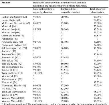
Table 2: Prediction results obtained with a neural network
Authors Best result obtained with a neural network and data taken from the most recent period before bankruptcy
Non-bankrupt firms Bankrupt firms Total of correct correctly classified correctly classified classification
Agarwal [40] 99.00% 93.70% 96.38%
Alfaro et al. [39] 92.37% 82.20% 87.29%
Altman et al. [9] 89.40% 86.20% 87.80%
Anandarajan et al. [42] 93.75% 95.45% 95.19%
Back et al. [11] 100.00% 98.00% 99.00%
Back et al. [26] 100.00% 94.25% 97.30%
Back et al. [27] 100.00% 94.40% 97.30%
Bell et al. [43] 97.70% 61.80% 94.00%
Berg [44] ? ? 69.50%
Boritz and Kennedy [45] 84.03% 74.27% ?
Bose and Pal [30] 75.62% 68.21% 71.88%
Boyacioglu et al. [38] ? ? 95.50%
Brabazon and Keenan [12] 82.67% 78.67% 80.67%
Brockett et al. [47] 94.50% 73.30% 89.30%
Charalambous et al. [31] 84.21% 84.21% 84.21%
Charitou et al. [48] 76.19% 90.48% 83.33%
Dorsey et al. [49] ? ? ?
Etheridge and Sriram [50] 92.71% 100.00% 92.85%
Fan and Palaniswami [51] ? ? 66.11%
Fanning and Cogger [52] 76.00% 94.00% 85.00%
Goss and Ramchandani [53]
75.00% 75.00% 75.00%
Huang et al. [54] ? ? ?
Jo et al. [55] ? ? 83.79%
Kim and McLeod [28] ? ? 78.70%
Kiviluoto [56] 88.30% 69.50% 86.50%
Kotsiantis et al. [57] ? ? 71.17%
Kumar et al. [8] ? ? 69.73%
Lacher et al. [82] 97.20% 91.50% 94.70%
Laitinen and Kankaanpaa [58]
89.50% 84.20% 86.80%
Lee et al. [59] ? ? 80.48%
Lee et al. [60] 76.19% 95.24% 85.22%
Table 2 – Continued
Authors Best result obtained with a neural network and data taken from the most recent period before bankruptcy
Non-bankrupt firms Bankrupt firms Total of correct correctly classified correctly classified classification
Leshno and Spector [61] 91.00% 90.90% 90.05%
Li and Gupta [62] ? ? 78.15%
McKee and Greenstein [63] 86.00% 75.00% 86.00%
Min et al. [64] ? ? 75.96%
Min and Lee [65] 85.71% 79.36% 82.54%
Min and Lee [66] ? ? 71.72%
Odom and Sharda [4] ? ? 81.81%
Pendharkar [67] ? ? ?
Piramuthu et al. [68] 92.70% 85.40% 89.10%
Pompe and Feelders [69] ? ? 72.60%
Salchenberger et al. [70] 90.00% 96.00% 92.50%
Sen et al. [32] ? ? ?
Serrano-Cinca [46] ? ? 93.94%
Sexton et al. [13] 97.40% 95.65% ?
Shin et Lee [71] ? ? 74.10%
Tam and Kiang [72] 85.00% 89.00% 87.00%
Tan and Dihardjo [73] 92.35% 64.70% 92.23%
Tung et al. [74] 99.31% 54.54% 73.12%
Tyree and Long [33] 100.00% 94.55% 97.95%
Vieira et al. [75] ? ? 90.00%
Wallrafen et al. [29] ? ? ?
West et al. [76] ? ? 87.27%
Wilson and Sharda [41] 98.00% 97.50% 97.75%
Wu et al. [77] 99.40% 83.30%
Yang and Harrison [83] 95.50% 92.37% 95.27%
Yang et al. [79] 90.00% 63.00% 84.00%
Yim and Mitchell [80] 94.00% 80.00% 90.96%
Yim and Mitchell [81] 100.00% 89.00% 96.55%
Table 3: Initial set of variables
Index Liquidity-Solvency
1 Current Assets/Current Liabilities 2 Current Assets/Total Assets
3 (Current Assets-Inventory)/Tot. Assets
4 Quick Ratio
5 Current Liabilities/Total Assets
6 Financial Debt/Cash Flow
7 (Cash+Mark. Sec.)/Total Sales 8 (Cash+Mark. Sec.)/Total Assets
9 EBITDA/Total Sales
10 Cash/Current Liabilities
11 Cash/Total Assets
12 Cash/Total Debt
Index Financial Structure
13 Net Op. Work. Capital/Total Assets 14 Shareholder Funds/Total Assets 15 Long Term Debt/Shareholder Funds 16 Long Term Debt/Total Assets 17 Total Debt/Shareholder Funds 18 Total Debt/Total Assets
Index Profitability
19 EBITDA/Permanent Assets
20 EBITDA/Total Assets
21 Profit before Tax/Shareholder Funds
22 EBIT/Total Assets
23 Net Income/Shareholder Funds 24 Net Income/Total Assets Index Efficiency
25 Total Sales/Shareholder Funds 26 Total Sales/Total Assets
27 Operating Cash Flow/Total Assets 28 Operating Cash Flow/Total Sales 29 Gross Trading Profit/Total Sales
30 EBIT/Total Sales
31 Value Added/Total Sales
Index Rotation
32 Current Assets/Total Sales 33 Net Op. Work. Capital/Total Sales 34 Accounts Receivable/Total Sales 35 Accounts Payable/Total Sales 36 Inventory/Total Sales
37 Cash/Total Sales
Index Withdrawal
38 Change in Other Debts
39 Change in Equity Position
Index Contribution
Table 3 – Continued
[image:27.595.127.470.257.700.2]41 Labor Expenses/Total Sales
Table 4: Characteristics of the variables belonging to the learning and valida-tion samples ( Means - Normality test and tests for differences between the two groups)
Mean Standard deviation S-W
Index B NB B NB B NB t U
Liquidity-Solvency
1 -0.46 0.46 0.69 1.05 0.000 0.000 0.000 0.000
2 0.12 -0.12 1.00 0.99 0.000 0.000 0.008 0.000
3 -0.46 0.46 0.54 1.14 0.000 0.000 0.000 0.000
4 -0.08 0.08 1.01 0.98 0.000 0.000 0.063 0.039
5 0.51 -0.51 1.17 0.33 0.000 0.024 0.000 0.000
6 0.02 -0.02 1.41 0.12 0.000 0.000 0.669 0.000
7 -0.48 0.48 0.48 1.15 0.000 0.000 0.000 0.000
8 -0.51 0.51 0.52 1.10 0.000 0.000 0.000 0.000
9 -0.55 0.55 0.99 0.64 0.000 0.000 0.000 0.000
10 -0.50 0.50 0.33 1.18 0.000 0.000 0.000 0.000
11 -0.53 0.53 0.75 0.94 0.000 0.095 0.000 0.000
12 -0.48 0.48 0.32 1.20 0.000 0.000 0.000 0.000
Financial Structure
13 -0.23 0.23 1.29 0.48 0.000 0.473 0.000 0.000
14 -0.54 0.54 1.15 0.29 0.000 0.000 0.000 0.000
15 -0.02 0.02 1.41 0.13 0.000 0.000 0.681 0.000
16 0.19 -0.19 1.28 0.54 0.000 0.000 0.000 0.000
17 -0.54 0.54 0.42 1.12 0.000 0.000 0.000 0.000
18 0.54 -0.54 1.16 0.30 0.000 0.000 0.000 0.000
Profitability
19 0.01 -0.01 1.41 0.04 0.000 0.000 0.743 0.000
20 -0.55 0.55 1.02 0.60 0.000 0.000 0.000 0.000
21 -0.13 0.13 1.37 0.29 0.000 0.000 0.003 0.000
22 -0.55 0.55 1.08 0.47 0.000 0.000 0.000 0.000
23 -0.02 0.02 1.41 0.05 0.000 0.000 0.651 0.026
24 -0.54 0.54 1.11 0.43 0.000 0.000 0.000 0.000
Efficiency
25 -0.07 0.07 1.41 0.09 0.000 0.000 0.142 0.000
26 -0.01 0.01 1.00 1.00 0.000 0.000 0.878 0.994
27 -0.23 0.23 1.17 0.72 0.000 0.000 0.000 0.000
28 -0.19 0.19 1.20 0.70 0.000 0.000 0.000 0.000
29 -0.14 0.14 1.04 0.94 0.000 0.005 0.001 0.006
30 -0.55 0.55 1.04 0.56 0.000 0.000 0.000 0.000
31 -0.35 0.35 0.94 0.94 0.000 0.001 0.000 0.000
Rotation
Table 4 – Continued
Mean Standard deviation S-W
Index B NB B NB B NB t U
32 0.10 -0.10 1.13 0.84 0.000 0.000 0.028 0.121
33 -0.20 0.20 1.25 0.60 0.000 0.000 0.000 0.000
34 0.16 -0.16 1.11 0.85 0.000 0.000 0.000 0.001
35 0.38 -0.38 1.20 0.52 0.000 0.000 0.000 0.000
36 0.18 -0.18 1.16 0.77 0.000 0.000 0.000 0.001
37 -0.51 0.51 0.75 0.96 0.000 0.000 0.000 0.000
Withdrawal
38 0.09 -0.09 1.17 0.78 0.000 0.000 0.046 0.000
39 0.04 -0.04 1.07 0.93 0.000 0.000 0.431 0.995
Contribution
40 0.07 -0.07 1.33 0.49 0.000 0.000 0.139 0.026
41 0.29 -0.29 0.97 0.95 0.000 0.000 0.000 0.000
S-W: p-value of a Shapiro-Wilks normality test
t: p-value of a Student t test for differences between the means of the two groups
U: p-value of a Mann-Whitney test for the equality of the sum of ranks of each group
B: Bankrupt NB: Non Bankrupt
[image:28.595.208.389.478.578.2]Index: the same as in Previous Table
Table 5: Selected variables using a Wilks Lambda criterion
Variables included into the model Freq.1 Cash/Total Assets 93.4% Total Debt/Shareholder Funds 91.1% Cash/Total Debt 88.7% (Cash+Mark. Sec.)/Total Assets 87.5% EBIT/Total Assets 81.2% EBITDA/Total Assets 76.8% Shareholder Funds/Total Assets 72.2%
Table 10: Rank of the variables according to an F test
Variables F p-val Rank1
1 EBIT/Total Sales 220.15 0.000 7
2 EBITDA/Total Sales 219.49 0.000
3 EBIT/Total Assets 218.96 0.000 3
4 EBITDA/Total Assets 213.91 0.000 1
[image:28.595.150.446.630.722.2]Table 10 – Continued
Variables F p-val Rank1
5 Net Income/Total Assets 210.01 0.000 7
6 Shareholder Funds/Total Assets 207.59 0.000 3
7 Total Debt/Total Assets 202.20 0.000 7
8 Total Debt/Shareholder Funds 201.14 0.000 7
9 Cash/Total Assets 195.01 0.000
10 Cash/Total Sales 179.60 0.000 7
11 Current Liabilities/Total Assets 179.32 0.000
12 (Cash+Mark. Sec.)/Total Assets 171.62 0.000 3
13 Cash/Current Liabilities 168.19 0.000 3
14 Cash/Total Debt 150.50 0.000
15 (Cash+Mark. Sec.)/Total Sales 145.63 0.000 16 Current Assets/Current Liabilities 133.77 0.000 7
17 Quick Ratio 131.30 0.000
18 Accounts Payable/Total Sales 85.95 0.000
19 Value Added/Total Sales 68.37 0.000
20 Change in Equity Position 44.29 0.000 1
21 Operating Cash Flow/Total Sales 28.57 0.000 7
22 Net Operating Working Capital/Total Assets 27.21 0.000 23 Net Operating Working Capital/Total Sales 21.10 0.000 24 Operating Cash Flow/Total Assets 19.40 0.000
25 Long Term Debt/Total Assets 19.32 0.000
26 Inventory/Total Sales 16.00 0.000
27 Accounts Receivable/Total Sales 13.38 0.000 7
28 Gross Trading Profit/Total Sales 10.53 0.001 29 Profit before Tax/Shareholder Funds 8.97 0.003
30 Current Assets/Total Assets 7.13 0.008
31 Current Assets/Total Sales 4.83 0.028
32 Financial Expenses/Total Sales 4.04 0.045
33 (Current Assets-Inventory)/Total Assets 3.47 0.063
34 Change in Other Debts 2.20 0.139
35 Total Sales/Shareholder Funds 2.16 0.142
36 Labour Expenses/Total Sales 0.62 0.431
37 Net Income/Shareholder Funds 0.20 0.651
38 Financial Debt/Cash Flow 0.18 0.669
39 Long Term Debt/Shareholder Funds 0.17 0.681
40 EBITDA/Permanent Assets 0.11 0.743
41 Total Sales/Total Assets 0.02 0.878
Table 6: Selected variables using a Likelihood criterion
(a)
Search: Backward Stepwise
Variables included into the model Freq. Shareholder Funds/Total Assets 94.0% Profit before Tax/Shareholder Funds 89.3% Change in Equity Position 87.6% (Cash+Mark. Sec.)/Total Assets 86.1% (Cash+Mark. Sec.)/Total Sales 81.5% EBITDA/Total Assets 73.9% Cash/Total Sales 70.2%
(b)
Search: Forward Stepwise
Variables included into the model Freq. Change in Equity Position 83.6% Shareholder Funds/Total Assets 81.2% Cash/Total Debt 77.3% EBITDA/Total Assets 72.1% EBIT/Total Sales 70.8%
Table 7: Selected variables using neural network criteria
(a)
Error
Variables included into the model Freq. Shareholder Funds/Tot. Assets 91.8% EBIT/Total Assets 86.2% Cash/Current Liabilities 83.1% Change in Equity Position 81.8% EBITDA/Total Assets 76.6% EBIT/Total Sales 76.1% (Cash+Mark. Sec.)/Tot. Assets 74.9% Accounts Receivable/Tot. Sales 70.6%
(b)
0 Order
Variables included into the model Freq. Net Income/Total Assets 86.7% (Cash+Mark. Sec.)/Tot. Assets 84.3% Shareholder Funds/Tot. Assets 83.8% EBITDA/Total Assets 80.9% Cash/Current Liabilities 78.2% Total Debt/Total Assets 74.5% Change in Equity Position 73.9% Cash/Total Sales 71.5%
(c)
1stOrder
[image:30.595.110.484.447.695.2]Table 8: Rank of the variables
Variables Number of Rank of appearance in
selections the six models
EBITDA/Total Assets 6 4 4 5 5 6 6
Shareholder Funds/Total Assets 5 1 1 2 3 7
Change in Equity Position 5 1 3 3 4 7
(Cash+Mark. Sec.)/Total Assets 4 2 4 4 7
EBIT/Total Assets 3 2 4 5
Total Debt/Shareholder Funds 2 1 2
Cash/Total Debt 2 3 3
Cash/Current Liabilities 2 3 5
EBIT/Total Sales 2 5 6
Cash/Total Sales 2 7 8
Net Income/Total Assets 1 1
Cash/Total Assets 1 1
Current Assets/Current Liabilities 1 2 Profit before Tax/Shareholder Funds 1 2
(Cash+Mark. Sec.)/Total Sales 1 5
Operating Cash Flow/Total Sales 1 6
Total Liabilities/Total Assets 1 6
[image:31.595.181.416.483.679.2]Accounts Receivable/Total Sales 1 8
Table 9: Rank of the variables selected with a neural network
Table 11: Model accuracy for ”modelling technique/variable selection method” pairs calculated on validation samples
DA LR LR NN NN NN Wilks-S Lik.-S Lik.-FS Error-B 0 order-B 1storder-B
NB 91.20% 93.60% 89.56% 92.78% 91.96% 92.82% B 83.20% 90.42% 88.84% 95.28% 95.22% 92.82% Total 87.20% 92.01% 89.20% 94.03% 93.59% 92.82% DA: Discriminant analysis, LR: Logistic regression, NN: Neural network Lik.: Likelihood, B: Backward, F: Forward, S: Stepwise
[image:32.595.139.459.310.412.2]NB: Non-bankrupt, B: Bankrupt
Table 12: Model accuracy for ”modelling technique/variable selection method” pairs calculated on test samples
DA LR LR NN NN NN Wilks-S Lik.-S Lik.-FS Error-B 0 order-B 1storder-B
NB 89.62% 91.15% 88.85% 93.08% 92.69% 91.15% B 80.77% 90.38% 88.46% 94.62% 91.92% 88.85% Total 85.19% 90.77% 88.65% 93.85% 92.31% 90.00% DA: Discriminant analysis, LR: Logistic regression, NN: Neural network Lik.: Likelihood, B: Backward, F: Forward, S: Stepwise
NB: Non-bankrupt, B: Bankrupt
Table 13: Model accuracy according to modelling techniques and two variable selection criteria (Wilks’s lambda-Likelihood) calculated on validation samples
Wilks’s lambda Likelihood Likelihood
Stepwise Backward stepwise Forward stepwise
DA LR NN DA LR NN DA LR NN
NB 91.20% 88.06% 90.02% 87.28% 93.60% 89.68% 87.98% 89.56% 88.08%
B 83.20% 79.18% 77.20% 84.84% 90.42% 92.74% 82.42% 88.84% 91.14%
Total 87.20% 83.62% 83.61% 86.06% 92.01% 91.21% 85.20% 89.20% 89.61%
DA: Discriminant analysis, LR: Logistic regression, NN: Neural network NB: Non-bankrupt, B: Bankrupt
Table 14: Model accuracy according to modelling techniques and three variable selection criteria (Error, 0 and 1st-order) calculated on validation samples
Error 0 Order 1stOrder
Backward Backward Backward
DA LR NN DA LR NN DA LR NN
NB 83.38% 90.44% 92.78% 83.20% 86.38% 91.96% 87.06% 88.16% 92.82%
B 85.38% 89.56% 95.28% 84.00% 89.64% 95.22% 81.84% 90.22% 92.82%
Total 84.28% 90.00% 94.03% 83.60% 88.01% 93.59% 84.45% 89.19% 92.82%
[image:32.595.106.500.463.534.2] [image:32.595.107.495.606.674.2]