Assessing the Risks of Trading Strategies Using Acceptability Indices

http://dx.doi.org/10.4236/jmf.2013.34049

Assessing the Risks of Trading Strategies Using

Acceptability Indices

Masimba E. Sonono1, Hopolang P. Mashele2

1_{Unit for Business Mathematics and Informatics, North-West University, Potchefstroom, South Africa} 2_{Centre for Business Mathematics and Informatics, North-West University, Potchefstroom, South Africa}

Email: [email protected], [email protected]

Received August 4,2013; revised September 30, 2013; accepted October 11, 2013

Copyright © 2013 Masimba E. Sonono, Hopolang P. Mashele. This is an open access article distributed under the Creative Commons Attribution License, which permits unrestricted use, distribution, and reproduction in any medium, provided the original work is properly cited.

ABSTRACT

The paper looks at the quantification of risks of trading strategies in incomplete markets. We realized that the no-arbi- trage price intervals are unacceptably large. From a risk management point of view, we are concerned with finding prices that are acceptable to the market. The acceptability of the prices is assessed by risk measures. Plausible risk measures give price bounds that are suitable for use as bid-ask prices. Furthermore, the risk measures should be able to compensate for the unhedgeable risk to an extent. Conic finance provides plausible bid-ask prices that are determined by the probability distribution of the cash flows only. We apply the theory to obtain bid-ask prices in the assessment of the risks of trading strategies. We analyze two popular trading strategies—bull call the spread strategy and bear call spread strategy. Comparison of risk profiles for the strategies is done between the Variance Gamma Scalable Self De-composable model and the Black-Scholes model. The findings indicate that using bid-ask prices compensates for the unhedgeable risk and reduces the spread between bid-ask prices.

Keywords: Conic Finance; Coherent Risk Measure; Acceptability Indices; Incomplete Markets; Bid-Ask Prices; Continuous Time Models

1. Introduction

The paper focuses on the quantification of risks of trad-ing strategies, particularly when the market is incomplete. The incompleteness of the market gives rise to many martingales, each of which produces a no-arbitrage price. Thus there is no exact replication so as to obtain a unique price. Furthermore, the no-arbitrage price intervals are unacceptably large. From a risk management point of view, we are concerned with finding the prices which are acceptable. The acceptability of these prices is assessed by risk measures.

In the financial literature, two major classes of risk measures have gained ground in assessing the risks of financial positions. Foremost, we have coherent meas-ures introduced by [1]. Since then, the theory of coherent risk measures has been applied to several problems in finance. Secondly, there is the grounding work of [2], in which they proposed a new class of performance meas-ures known as acceptability indices. The acceptability indices can be considered as an extension of coherent risk measures. Under the acceptability framework, a

fi-nancial position is acceptable if its distribution function withstands high levels of stress, or in other words, a stressed sampling of the financial position has a positive expectation. In this paper, our contribution is assessing the risk profiles of trading strategies using the acceptabil-ity framework.

The rest of the paper is organized as follows: Section 2 looks at the problem of pricing in incomplete markets. Section 3 gives an overview of risk measures and pre-sents new acceptability indices based on the family of distortion functions. Section 4 presents a brief detail on conic finance and provides closed form expressions for the bid-ask prices. Section 5 presents the models that are used in this work. Section 6 presents numerical tests on assessing the risks of two trading strategies. Section 7 is the conclusion.

range of values of a risky position payoff. Let be the set of replicable payoffs, be the market price to replicate a payoff Y , and

R

 

Y



R

 A be an acceptance set of

payoffs that are acceptable to the situation. The lower good deal bound for a payoff X is:

 

sup



 

.

Y R

b X Y Y X A



   



(1)

This payoff might be interpreted as a bid price. Equa-tion (1) tells us that if X can be bought for less than

, then there is a that can be bought for

 

b X Y 

 

Y

such that a cost . The upper good deal bound, which might be interpreted as the ask price for

 

 

0

b X   Y 

X, is given by:

 

 

inf



 



.

Y R

a X b x Y Y X A



       (2) Equation (2) tells us that selling X or buying X

yields the same effect. The interpretation of b X

 

is

the cost that renders X to be acceptable. As [5]

pro-pose: any valuation principle that gives price bounds induces a risk measure and vice versa. The accept- ance set A must include the set of riskless payoffs,



Z Z0



, which is the acceptance set that generates no-arbitrage bounds. The set A does not intersect with

the set



Z Z 0



of pure losses. The acceptance set

A must be consistent with market prices, , or

arbi-trage occurs.



Now, an incomplete market is one in which there are many martingale measures . The price bounds in Equations (1) and (2) form an interval of arbitrage-free prices for

Q

X:

 

 

inf Q , sup Q

Q _Q

I E X E X

 _

  

  _

 

 (3)

where is a set of equivalent martingale measures. The problem with the interval of the arbitrage-free prices for



X is that it is usually too wide for the no-arbitrage

bounds to serve as useful bid-ask prices.

In practice, derivatives traders are aware of the incom-pleteness of the markets and after making trades on cer-tain positions, they are not able to hedge away all the risk. Instead, they must bear the risk associated with the trade. To cover their business expenses and to earn compensa-tion for bearing the risk they are not able to hedge, trad-ers establish bid-ask intervals around the expected dis-counted payoff.

Now, in constructing the bid-ask prices, the difficulty posed by incomplete markets is very significant because of adverse selection. For instance, if the ask price is too high, few potential investors will be willing to pay so much and the result is foregone profits. If the ask price is too low, the resulting trade is bad for a trader and entails likely losses. So, to ensure that trades made at bid and ask prices are beneficial, it helps to use methods that produce bounds for the prices that are suitable for use as

bid-ask prices and are adequate to minimize unhedgeable risk to an extent. In the process, we will be able to quan-tify risk since any valuation method that yields price bounds also induces a risk measure [5].

3. Risk Performance Measures

In this section, we give a brief overview of the risk measures. In general, a risk measure, :X , is a

functional that assigns a numerical value to a random variable representing an uncertain payoff.

3.1. Coherent Risk Measure

Definition Coherent Risk Measure

A risk measure  is coherent if it satisfies the follow-ing axioms:

 Translation Invariance:



X r



 

X

   ,

for allX,.

 Monotonicity: 

 

X 

 

Y if X Y a.s.

 Positive Homogeneity:



X



 

X

   ,

for  0.

 Subadditivity:



X Y



 

X

 

    Y ,

for all X Y, 

 Relevance: 

 

X 0 if X 0 and X 0.

The last property is included although it is not a de-terminant of coherency. Translation invariance axiom implies that by adding a fixed amount  to the initial position and investing it in a reference instrument, the risk

 

X

 decreases by  . The monotonicity axiom pos-tulates that if X

 

 Y

 

 for every state of nature,

is more risk because it has higher risk potential.

Y

The positive homogeneity axiom implies that risk linearly increases with size of the position, that is to say that the size of the risk of a position should scale with the size of the position. This is just a natural requirement, though this condition may not be satisfied in the real world since markets may be illiquid. The subadditivity axiom implies that the risk of a portfolio is always less than the sum of the risks of its subparts. This axiom en-sures that diversification decreases the risk.

According to the basic representation theorem proved by[1] for a finite  , any coherent risk measure admits a representation of the form:

 

inf Q

 

Q

X E X



  

 , (4) with a certain set of probability measures with respect to . A cash flow



P X is acceptable if it has negative risk,

3.2. Acceptability Indices

Cherny and Madan, defined a subclass of risk measures called acceptability indices, defined formally as:

3.3. Definition. Index of Acceptability

The acceptability index is as a mapping  from the set of bounded random variables to the extended half-line

 

0, . The index satisfies the following four properties:

 Monotonicity

If Y dominates X, that is X Y, then

 

X

 

Y

  .

 Scale invariance

 

X

 stays the same when X is scaled by a

posi-tive number, that is 

 

cX 



X



for c0.

 Quasi-concavity

If 

 

X Y and

 

Y Y, then







X 1 Y



Y

     ,

for any  

 

0,1 .

 Fatou Property (Convergence)

Let

 

Xn be a sequence of random variable.

1

n and

X  Xn converges in probability to a random variable X. If 

 

Xn x, then 

 

X x.

The acceptability indices are constructed by replacing the cumulative distribution function of X,FX

 

x



, by a

risk adjusted distribution, X



FX

 

x . The corre-sponding risk measure is the negative expectation of the zero cost cash flow under the distorted distribution func-tion:

 

X xd





FX

 

x





,

 

  

_

  _

   (5) where _ is a family of concave distortion functions on [0,1] increasing pointwise in the stress level parameter . A higher value of  results in severe distortion of the distribution function of X. Then, the acceptability index,

 

X

 , is the largest stress level  such that the expec-tation of X remains positive under the distortion or in

other words the distorted cash flow remains acceptable:

 

X sup



: 

 

X 0 .



  _   (6) Cherny and Madan introduced four acceptability indi-ces based on the family of distortion functions which are namely: AIMIN, AIMAX, AIMINMAX, AIMAXMIN.

 AIMIN is the largest number x such that the

expec-tation of the minimum of x1 draws from cash flow distribution is still positive. Let

1 1

min , , law

x

Y  X  X  ,

where X1, , Xx1 are independent draws from X.

The concave distortion function is given by:

 





1

 

1 1 x , , 0,1

x y y x y

 

      (7)

 AIMAX constructs a distribution from which one draws numerous times and takes the maximum to get the cash flow distribution being evaluated. Let,



1 1



max Y, ,Yx law X

1

,

where Y₁, ,Yx are independent draws of . The

concave distortion function is given by:

Y

 

x11_{, ,}

 

_0,

x y y x y

 

    1



1

(8)

 AIMAXMIN is constructed by first using the MIN-VAR and then followed by the MAXMIN-VAR to create worst case scenarios.

Let



1 1





1

max Y, ,Yx lawmin X , , Xx

, ,

,

where X1 Xx1 are independent draws of X and 1, , x 1

Y Y_ are independent draws of . Combining

the MINVAR and MAXVAR, we have the distortion function:

Y

 







1



1₁

 

, 1 1 x _x , 0,1

x y y x y

 _{ }

      (9)

 AIMAXMIN is constructed by first using the MAXVAR and then followed by the MINVAR to create worst case scenarios. Let

1 1

min , , ,

law

x

Y  Z  Z _

law

1 1

max , ,Z  Zx  X, , ,

where Z₁ Z_x1 are independent draws of Z .

Combining the MINVAR and MAXVAR, we have the distortion function:

 

 

1 1

1

1 1 , , 0,

x

x

x y y x y



 

 

 

 



 



     1 (10)

The acceptability indices are more plausible in assess-ing the risks of financial positions. The acceptability in-dices have been used heavily in the theory of conic fi-nance, which we review next.

4. Conic Finance Theory

We look at the principles of conic finance as set out in [6]. The market serves a passive counterparty accepting the opposite side of zero cost trades proposed by market participants. The departure of conic finance from the traditional one price economy is that trade now depends on the direction of trade, with the market buying at bid price and selling at ask price. Cash flows to trade are modeled as bounded random variables on a fixed prob-ability space



, , P



for a base probability measure

selected by the economy.

the random variable X with a distribution F x

 

Q

at a fixed period, we develop bid-ask prices at which the cash flow is bought and sold such that the net cash flow is an acceptable risk. The set of acceptable risks is defined by a convex cone of random variables that contains the non-negative cash flows. [1] showed that any acceptable set (cone) of acceptable risks, there exists a convex set of probability measures , equiva-lent to , with the property that if and only if:



 Q

X P

 

0, all .

Q

E X  Q (11)

The acceptability of a cash flow can then be com-pletely determined by its distribution function. Accept-ability of cash flows is linked to positive expectation via concave distortion. So for some concave distribution function , the cash flow distribution function

 

u



 

0



 u 1



F x P Xx



is acceptable if:

 





d

x F x

  



0. (12) [6] show that the bid price, b x

 

, for the cash flow X

is given by:

 

d



 



0 inf Q

 

Q

b x  x F x E X

 



_

  

 ,





(13) and the ask price is given by:

 

d



1

 



0 sup Q

 

.

Q

a x  x F x E X

 _

 

_

     

(14)

The bid and ask prices for call and put options can be obtained by using closed formulas which are obtained on integration by parts. Let be the random variable at time of an underlying asset. The call option

and put option , where

S T



 

C S K  P



KS  K

is the strike price. The following are the closed bid and ask prices expressions:

 

_K



1 S

 



a_ C 



 F x d ,x



d ,

.

(14)

 

_K



1



S

 



b C_ 



   F x x (15)

 

₀K



_S

 



d ,

a P 



 F x x (16)

 

0



1



1

 





d

K

S

b_ P 



  F x x (17)

s

F is the distribution function of and is important

because the bid and ask prices are determined completely by this distribution.

S

5. Continuous Time Models for Option

Pricing

This section looks at the models that are used for option pricing. It is acknowledged that the relatively most liquid traded assets with market information are quoted vanilla options. In practice, trades mark to market their models

to quoted vanilla options before they can price non- quoted options. As a result, this has led to demands for models that are capable of synthesizing the surface of vanilla options. It is well known that the geometric Brownian model is not capable of synthesizing the sur-face of vanilla options, although it remains a standard quoting model in the markets. Improvements on this model are offered by Lévy processes, which were found to be successful in synthesizing across strikes for a given maturity. The following is a brief overview of the mod-els.

5.1. Black-Scholes Model

The log-normal process models continuously compound- ed returns using the general Brownian motion so that:

 

 

,

X t tW t (18)

where W t

 

is a standard Weiner process,  is the

instantaneous drift and  is the instantaneous volatility of returns. The stochastic differential equation of the stock price is:

 

 



 



dS t S t dtdW t , (19)

where  is the growth rate of the stock and is related to

 as follows _{  1 2}2 _{. The stochastic differential} equation can be solved to give the following dynamics of the stock price:

 

 

_{0 exp} 1 2

 

2

S t S _  _tW t 

 . (20)

The characteristic function for the logarithm of the stock price is:

 

 

_{ }

ln 1 2 1 2

e exp ln 0

2 2

iu S t

E_  _ _iu_ S _  __t  u t2 _

 

 

 

(21)

5.2. Variance Gamma Model

[7] define a Variance Gamma process, X t



, , ,  



, as

a time changed Brownian motion as follows:



, , ,



 



 



,

X t    t W  t (22)

where 

 

t is a Gamma process with parameters

and , that is,

a b 

 

t ~Gamma at b



 

a b,

 ,



where the gamma

probability density function is given by:



, ,



_{ }

1e , 0.

a a bx

b x

f x a b x

a



 

 

 (23)

 and  are respectively the instantaneous drift and volatility and W t

 

is a standard Brownian motion.

a Variance Gamma process is known in closed form and requires the computation of the modified Bessel function of the second kind which can be time consuming. Thus we resort to using the characteristic function, which is found by the conditioning on the jump 

 

t as in many

Lévy processes and is given by:

 

 

2 2

t

u

1

1 .

2 X t u iu

           

  (24)

The dynamics of the stock price are given by:

 

 

0 exp









, , ,





,

S t S   tX t   (25)

where  is the instantaneous expected return of the stock evaluated at calendar time and  is a compensa-tor term The characteristic function for the logarithm of stock price is:

 

 

_

_{  }

_

_

 

 

ln

eiu S t exp ln 0

X t

E_{ }  iu_ S    t_  u .

(26) The compensator term can be found from the charac-teristic function and is given by:

 

 





1_ln

X t i

t

   .

5.3. Variance Gamma Scalable Self Decomposable (VGSSD) Model

Sato process model was first introduced by [8]. The Sato process was shown to be effective in synthesizing many options on numerous underliers at the same time. The idea behind the model was to construct stochastic proc-esses that had inhomogeneous independent increments from Lévy processes with homogeneous independent increments such that the higher moments are constant over the time horizon.

The starting point for the construction of the Sato model is the self-decomposable law. Loosely speaking, the self-decomposable law describes random variables that decompose into the sum of a scaled down version of themselves and an independent residual term. The scal-ing property means the distribution of increments of var-ious time scales can be obtained from that of other time scale by rescaling the random variable at that time scale. Thus the distribution at larger time scales are derived from those at smaller time scales, which are easier to estimate as the data are sufficient. [9] proposed that the self-decomposable law is associated with the unit time distribution of self-similar additive process whose in-crements are independent, but not necessarily stationary. It is known that stock prices are moved by many pieces of information. If the pieces of information are considered as a sequence of independent random vari-ables , then the price changes are

con-sequences of the impacts from all i



Zi:i1, 2,



Z . Now, let

0

n i

i

S 



Z denote their sum. Suppose that there exist

centering constants n and scaling constants bn such that the distribution of n n n converges to the dis-tribution of the random variable

c

b S c

X, which belongs to a

family law “class L”. Then the random variable X is

said to have the class L property. So, the price change over the time horizon is the outcome of many independ-ent random variables which can be approximated as a random variable X that has the law of “class L”. [10]

define the self-decomposable law as follows.

5.4. Definition Self Decomposable Law

A random variable X is self-decomposable if for all

 

0,1

c ,

,

law

c

X cXX (27)

where c

X is a random variable independent of X.

The self-decomposable random variable X can be

decomposed into a partial of itself and another inde-pendent random variable. [10] also shows that one may associate with such a self-decomposable law at unit time a process with independent but inhomogeneous incre-ments by defining the marginal law of the process at time points upon scaling the law at unit time. Therefore we have that:

t

 

X t t X t , 0. (28)

Thus we can study the price changes easily using self-decomposable laws, which are easier to handle than class L.

Self-decomposable laws are an important sub-class of the class of infinitely divisible laws [11]. The character-istic function of the self-decomposable laws has the form (see [10])

 

2 2 _eiux R

u 1

xp 1 1_x g x ,

E i iux x

x 

1 2

ru 

eiux e   _d      _   



_   __    (29) wherer, are constants, 20,



2



 

R

g x

x

1 d

x  x 



,

and g x

 

is an increasing function when x0 and

decreasing function when . An infinitely divisible law is self-decomposable if the corresponding Lévy den-sity has the form

0

x

 

g x

x ,

where g x

 

is increasing for negative x and

de-creasing for positive x.

 

 

0 exp



 

 

 

,

S t S r t X t  t



(30)

where is a compensator term. The Sato process used in this work is the one constructed from the vari-ance gamma process and is known as the Varivari-ance Gamma Scalable Self Decomposable (VGSSD) process. The variance gamma process is defined by time changing an arithmetic Brownian motion with drift

 

t



 and volatil-ity  by an independent gamma process with unit mean rate and variance rate  . Let G t



;



be the

gamma process, then the variance gamma process is written as:



, , ,



 

;





; , VG

X t    G t W G t





(31)

where is an independent standard Brownian mo-tion.

 

W t

The gamma process is an increasing pure jump Lévy process with independent identically distributed incre-ments over regular non overlapping intervals of length

that are gamma distributed with density

h fh

 

g

where:

 

1

e _{, 0}

h g

h h

v

g

f g g

h

 

    

     

.

 (32)

The VGSSD is constructed from the variance gamma process by defining the scaled stochastic process X t

 

such that it is equal in law to t XVG

 

1 where



_{ }

₁

VG

X

is a variance gamma random variable at unit time. It fol-lows that the characteristic function of X t

 

is given

by [7]

 

 

 1 2 2

1

1 .

2

VG

X t u X iut u t

_ _

 

    _  _

  (33) Since the VGSSD is a scaled stochastic process, its higher moments remain constant over time.

6. Numerical Tests

Next, focus is shifted to analyzing the risk profiles of option investing strategies. We examine two option strategies which are namely bull call spread strategy and bear call spread strategy. We determine the maximum risk, maximum reward and breakeven price for each of the strategies. Comparison of risk profiles is done be-tween the VGSSD model and the Black-Scholes model. The Black-Scholes model is considered here since it is the one that is mostly used by industrial practioners. So, the Black-Scholes is a proxy for market prices. The the-ory of conic finance provides bid-ask prices, which de-pend on the risk appetite of investors. For evaluation of bid-ask prices, we use acceptability indices based on the MAXMINVAR. The options used in the strategies are of

European type and are applied to Single Stocks Futures (SSF) options offered in the South African financial markets.

A bull call spread is a bullish strategy formed by buy-ing an “in-the-money call option” (lower strike) and sell-ing “out-of-the-money” (higher strike). Both call options must be on the same underlying and expiration date. The strategy’s net effect is to bring down the cost and break-even (long call strike price + net debt) on a buy call (long call) strategy.

A bear call spread is a bearish strategy formed by buy-ing an “out-of-the-money” call option (higher strike) and selling an “in-the-money” call option (lower strike). Both call options must be on the same underlying security and expiration date. The strategy's concept is to protect the downside of the sold call option by buying a call option of higher strike price. Then, the investor receives a net credit since the call option which has been bought has a higher strike price than the sold option. The breakeven will be the sum of the strike price of the short call option plus the premium received.

For numerical illustration purposes, we used names of two large South African banks—ABSA and Standard Bank. Note that, the illustrations do not pertain to any real positions on the banks. The bid-ask prices were computed at various theoretical prices of the underlying on the expiration date. The 3-month JIBAR is used as a proxy for the risk-free interest rate. To realize model calibration, we need market prices. Simulated data set of bid-ask options at different strikes maturing on the same date were generated using the models introduced in the previous Section.

The illustrations that follow merely suggest what an investor can do given the different risk appetites on an investor. The illustrations are implemented at stress (risk) level of 0.01, 0.05 and 0.10.

6.1. Bull Call Spread Risk Profile

6.1.1. Scenario

An investor owns 100 shares in ABSA Bank (ASAQ), which in early July are trading at a Single Stock Future (SSF) fair value of R140. The investor believes the mar-ket will be bullish in the coming 6 months and decided to create a bull call spread. So the investor buys a DEC ASAQ 140 call option and sells a DEC ASAQ call op-tion with a higher strike price, so as to create the bull call spread strategy. The concern for the investor is on the appropriate higher strike which can create an attractive strategy.

1) At different stress (risk) levels, the investor deter-mines the bid-ask prices for the range of strike prices.

2) The investor analyzes the risk profiles at each strike price choice so as to create an appropriate trade.

strategy, given a range of possible values of the underly-ing at expiration for the appropriate strike price from step 2 at a stress level of 0.01.

In addition, the investor gathers the following infor-mation:

3month JIBAR rate 5.01% Time to expiration 612 yr Dividend yield 0% (assumption).

In order to create the strategy appropriately, the inves-tor implemented the following steps.

1) Bid-Ask Prices at Different Stress

 

γ Levels The calibrated parameters used for this strategy are

0.240

  in the Black-Scholes model and

0.226, 0.131, 0.08, 0.480

       

in the VGSSD model. An attractive bull call spread is created when an investor buys a lower strike call and sells a higher strike call. In the scenario presented above, the investor has the choices shown in Table 1. Table 2 shows the bid-ask prices for the options using both the Black-Scholes model and VGSSD model.

2) Risk Profile Analysis

Next, we look at the risk profiles for each of the choices using bid-ask prices provided in step 1 at a stress level of 0.01. Under the Black-Scholes model, an attractive strategy can be created by choice 4) as shown in Table 3. The reason is that the risk and breakeven point is lower whilst maximum reward and maximum Return on Investment (ROI) are high enough to be at-tractive.

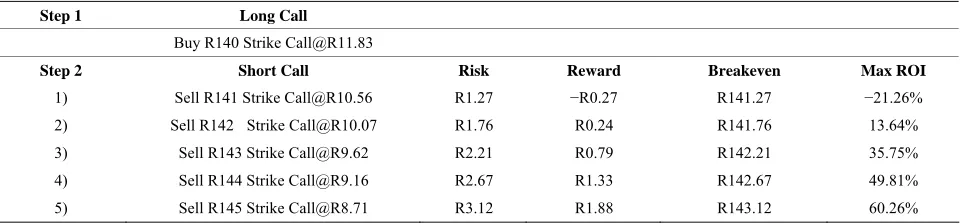
Also under the VGSSD model, an attractive strategy can be created using choice 4) as shown in Table 4. The reason being again that the risk and breakeven is lower whilst the maximum reward and maximum Return on Investment (ROI) are high enough to be attractive.

3) Scenario Analysis at the Expiration Date

After choosing an attractive choice from step 2, we now look at the profit/loss of the strategy at expiration for a range of prices for the underlying. We compare the profit/loss under the two models—Black-Scholes model and VGSSD model. Table 5 shows the profit/loss of the strategy under the two models. Figure 1 shows the plot of the profit/loss of the strategy for a range of prices of the underlying at expiration. From Figure 1, it can be observed that the breakeven point is lower using the VGSSD model than the Black-Scholes model. A lower breakeven point is ideal for a strategy which intends to reduce risk.

6.1.2. Comment on the Strategy

The spread was observed to be lower in the VGSSD model than in the Black-Scholes model. Reduced spread can minimize the unhedgeable risk, which can be a major

Table 1. Bull call spread investor choices.

Step 1 Long Call Buy R140 Strike Call

Step 2 1) Short Call Sell R141 Strike Call Or 2) Short Call Sell R142 Strike Call Or 3) Short Call Sell R143 Strike Call

Or 4) Short Call Sell R144 Strike Call

Or 5) Short Call Sell R145 Strike Call

boost for option trading strategies. As a result, the cost of trade is lowered as the sold options can offset the cost of the bought option. In conclusion, the strategy becomes less risky in terms of lower risk and lower breakeven point but offers limited potential reward, which can still be highly attractive.

6.2. Bear Call Spread Risk Profile

6.2.1. Scenario

In early July an investor believes the SSF fair price of Standard Bank (SBKQ) is going to fall from the current levels of R120 to around R117.50. The investor wants to create an attractive bear call spread. So the investor writes a SEP SBKQ 119 call option and buys a higher SEP SBKQ strike call, so as to create a bear call strategy. A little bit of concern to the investor is on the appropriate higher strike to choose so as to create an attractive strat-egy.

1) Now at different stress (risk) levels, the investor determines the bid-ask prices for the range of higher strike prices.

2) The investor analyzes the risk profiles at each of strike price choices so as to create an appropriate trade.

3) Finally, the investor accesses the performance of the strategy for the appropriate strike price in step 2 at a stress level of 0.01 given a range of possible values of the underlying at expiration.

1) Bid-Ask Prices at Different Stress

 

γ Levels The calibrated parameters used for this strategy are

0.306

  in the Black-Scholes model and

0.285, 0.070, 0.060, 0.510

      

in the VGSSD model. An attractive bear call spread is created when an investor sells a lower strike call and buys a higher strike call. In the scenario presented here, the investor has the choices shown in Table 6. Table 7 shows the bid-ask prices for the options using both the Black-Scholes model and VGSSD model.

2) Risk Profile Analysis

[image:8.595.59.538.100.358.2]

Table 2. Bull call spread bid-ask prices at different stress levels.

Black-Scholes Model VGSSD Model

Stress

Level _{S K Bid Ask Spread S K Bid Ask Spread}

0.01 140 140 11.05 11.83 0.78 140 140 11.04 11.77 0.73

141 10.56 11.32 0.76 141 10.54 11.25 0.71

142 10.07 10.81 0.74 142 10.04 10.73 0.69

143 9.62 10.33 0.71 143 9.59 10.26 0.67

144 9.16 9.85 0.69 144 9.15 9.79 0.64

145 8.71 9.37 0.66 145 8.70 9.32 0.62

0.05 140 140 10.50 14.59 4.09 140 140 10.49 14.28 3.79

141 10.03 14.00 3.79 141 10.01 13.68 3.67

142 9.56 13.40 3.84 142 9.53 13.09 3.56

143 9.09 12.80 3.71 143 9.07 12.52 3.45

144 8.67 12.28 3.61 144 8.66 12.01 3.35

145 8.24 11.72 3.48 145 8.23 11.47 3.24

0.10 140 140 9.85 18.45 8.60 140 140 9.81 17.67 7.86

141 9.38 17.72 8.34 141 9.35 16.99 7.64

142 8.93 17.03 8.10 142 8.92 16.35 7.43

143 8.49 16.33 7.84 143 8.46 15.67 7.21

144 8.07 15.67 7.60 144 8.05 15.05 7.00

[image:8.595.54.540.387.490.2]

145 7.68 15.05 7.37 145 7.67 14.46 6.79

Table 3. Bull call spread risk profile using Black-Scholes model.

Step 1 Long Call

Buy R140 Strike [email protected]

Step 2 Short Call Risk Reward Breakeven Max ROI

[image:8.595.59.539.517.629.2]

1) Sell R141 Strike [email protected] R1.23 -R0.23 R141.23 −18.70% 2) Sell R142 Strike [email protected] R1.73 R0.27 R141.73 15.61% 3) Sell R143 Strike [email protected] R2.18 R0.82 R142.18 37.61% 4) Sell R144 Strike [email protected] R2.62 R1.38 R142.62 52.67% 5) Sell R145 Strike [email protected] R3.07 R1.93 R143.07 62.87%

Table 4. Bull call spread risk profile using VGSSD model.

Step 1 Long Call

Buy R140 Strike [email protected]

Step 2 Short Call Risk Reward Breakeven Max ROI

1) Sell R141 Strike [email protected] R1.27 −R0.27 R141.27 −21.26% 2) Sell R142 Strike [email protected] R1.76 R0.24 R141.76 13.64% 3) Sell R143 Strike [email protected] R2.21 R0.79 R142.21 35.75% 4) Sell R144 Strike [email protected] R2.67 R1.33 R142.67 49.81% 5) Sell R145 Strike [email protected] R3.12 R1.88 R143.12 60.26%

a result choice 4) is attractive to create the strategy since the net credit is fairly high, and the breakeven point as well as the risk are reduced.

In Table 9 a potential strategy again can be created using a strike which provides reduced risk and lower breakeven. Also, the gain on this strategy is the net credit received upon entering the trade. As a result choice 4) is attractive to create the strategy since the net credit is

fairly high, and the breakeven point is reduced and the risk is fairly low.

3) Scenario Analysis at the Expiration Date

Table 5. Bull call spread profit/loss under Black-Scholes and VGSSD models.

Black-Scholes Model VGSSD Model

ASAQ@expiry Profit/Loss ASAQ@expiry Profit/Loss

135 −2.67 135 −2.62

136 −2.67 136 −2.62

137 −2.67 137 −2.62

138 −2.67 138 −2.62

139 −2.67 139 −2.62

140 −2.67 140 −2.62

141 −1.67 141 −1.62

142 −0.67 142 −0.62

[image:9.595.58.538.100.346.2]

142.67 0.00 142.62 0.00 143 0.33 143 0.38 144 1.33 144 1.38 145 1.33 145 1.38 146 1.33 146 1.38 147 1.33 147 1.38 148 1.33 148 1.38 149 1.33 149 1.38 150 1.33 150 1.38

Table 6. Bear call spread investor choices.

Step 1 Short Call Sell R119 Strike Call

Step 2 1) Long Call Buy R120 Strike Call

Or 2) Long Call Buy R121 Strike Call

Or 3) Long Call Buy R122 Strike Call

Or 4) Long Call Buy R123 Strike Call

[image:9.595.61.538.477.734.2]

Or 5) Long Call Buy R124 Strike Call

Table 7. Bear call spread bid-ask prices at different stress levels.

Black-Scholes Model VGSSD Model

Stress

Level _{S K Bid Ask Spread S K Bid Ask Spread}

0.01 120 119 6.91 7.45 0.54 120 119 6.87 7.40 0.73

120 6.40 6.90 0.50 120 6.37 6.86 0.71 121 5.92 6.40 0.48 121 5.88 6.35 0.69 122 5.47 5.93 0.46 122 5.43 5.89 0.67 123 5.02 5.45 0.43 123 5.01 5.43 0.64 124 4.62 5.03 0.41 124 4.61 5.02 0.41

0.05 120 119 6.57 9.42 2.85 120 119 6.55 9.34 2.79

120 6.06 8.76 2.70 120 6.04 8.67 2.63 121 5.61 8.16 2.55 121 5.59 8.09 2.50 122 5.18 7.61 2.43 122 5.17 7.53 2.36 123 4.75 7.03 2.28 123 4.73 6.95 2.22 124 4.35 6.50 2.15 124 4.33 6.42 2.09

0.10 120 119 6.16 12.25 6.09 120 119 6.14 12.05 5.91

120 5.67 11.44 5.77 120 5.66 11.28 5.62 121 5.25 10.74 5.49 121 5.23 10.56 5.33

122 4.81 10.00 5.19 122 4.80 9.85 5.05

[image:10.595.58.543.100.205.2]

Table 8. Bear call spread risk profile using Black-Scholes model.

Step 1 Short Call

Sell R119 Strike [email protected]

Step 2 Long Call Risk Reward Breakeven Max ROI

1) Buy R120 Strike [email protected] R0.99 R0.01 R119.01 1.01%

2) Buy R121 Strike [email protected] R1.49 R0.51 R119.51 34.23% 3) Buy R122 Strike [email protected] R2.02 R0.98 R119.98 48.51% 4) Buy R123 Strike [email protected] R2.54 R1.46 R120.46 57.48%

[image:10.595.55.289.233.651.2]

5) Buy R124 Strike [email protected] R3.12 R1.88 R120.88 60.26%

Table 9. Bear call spread risk profile using VGSSD model.

Step 1 Short Call

Sell R119 Strike [email protected]

Step 2 Long Call Risk Reward Breakeven Max ROI

1) Buy R120 Strike _{[email protected]} R0.99 R0.01 R119.01 1.01%

2) Buy R121 Strike _{[email protected]} R1.48 R0.52 R119.52 35.14%

3) Buy R122 Strike _{[email protected]} R2.02 R0.98 R119.98 48.51%

4) Buy R123 Strike _{[email protected]} R2.56 R1.44 R120.44 56.25%

[image:10.595.57.289.233.644.2]

5) Buy R124 Strike _{[email protected]} R3.15 R1.85 R120.85 58.73%

Figure 1. Plot of bull call spread profit/loss.

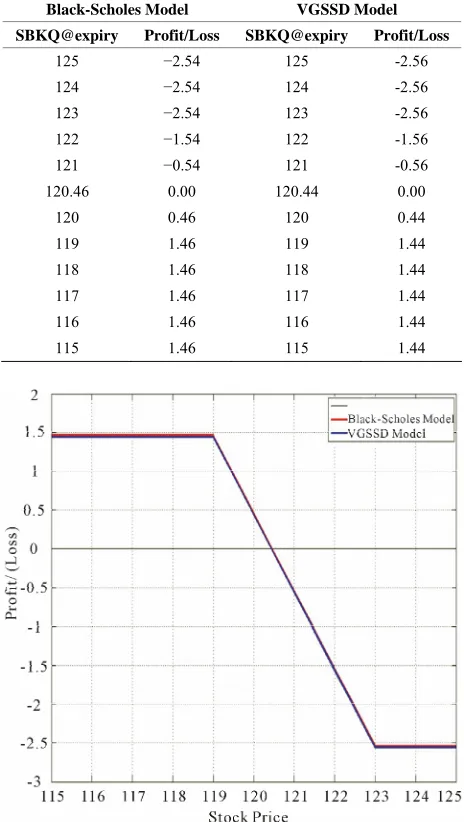
two models. Figure 2 shows the plot of the profit/loss of the strategy for a range of prices of the underlying at ex-piration. The breakeven point is lower in the VGSSD model than the Black-Scholes model, which is ideal in creating a strategy with reduced risk.

Table 10. Bull call spread profit/loss under the Black-Scho- les and VGSSD models.

Black-Scholes Model VGSSD Model

SBKQ@expiry Profit/Loss SBKQ@expiry Profit/Loss

125 −2.54 125 -2.56

124 −2.54 124 -2.56

123 −2.54 123 -2.56

122 −1.54 122 -1.56

121 −0.54 121 -0.56

[image:10.595.306.539.242.664.2]

120.46 0.00 120.44 0.00 120 0.46 120 0.44 119 1.46 119 1.44 118 1.46 118 1.44 117 1.46 117 1.44 116 1.46 116 1.44 115 1.46 115 1.44

Figure 2. Plot of bear call spread profit/loss.

6.2.2. Comment on the Strategy

[image:10.595.307.539.245.656.2]

point. However, in this strategy reducing the risk impacts on the potential reward under the VGSSD model as compared to the Black-Scholes model.

7. Conclusions

In this paper, we have looked at the quantification of risks of trading strategies in incomplete markets. We established that the no-arbitrage price intervals are unac-ceptably large. We need intervals with prices which are acceptable to the market. The acceptability of the prices is assessed by risk measures. Ideal risk measures are those that produce price bounds that are suitable for use as bid-ask prices and are able to compensate for un-hedgeable risk. Plausible risk measures we look at are coherent risk measure and acceptability indices. Accept-ability indices are heavily used in the theory of conic finance, which we used to assess the risk of trading strategies. Conic finance provides plausible bid-ask pric-es which are determined only by the probability distribu-tion of the cash flow.

We assess the risks of financial positions using two strategies-bull call spread and bear call spread. Com-parison of the risk profiles for the trading strategies is done between the VGSSD model and the Black-Scholes model. The findings showed that the spread was reduced, especially using the VGSSD model as compared to the Black-Scholes model. In addition, the findings showed that the bid-ask price intervals are able to compensate for the unhedgeable risk. Ultimately, reward from the strate-gies had a potential of increasing.

REFERENCES

[1] P. Artzner, F. Delbaen, J. Eber and D. Heath, “Definition of Coherent Measure of Risk,” Mathematical Finance, Vol. 9, No. 3, 1999, pp. 203-228.

http://dx.doi.org/10.1111/1467-9965.00068

[2] A. Cherny and D. Madan, “New Measure of Performance Evaluation,” Review of Financial Studies, Vol. 22, No. 7, 2009, pp. 2571-2606.

http://dx.doi.org/10.1093/rfs/hhn081

[3] J. N. Cochrane and J. Saá-Requejo, “Beyond Arbitrage: ‘Good Deal’ Asset Price Bounds in Incomplete Markets,”

Journal of Political Economy, Vol. 108, No. 1, 2000, pp.

79-11. http://dx.doi.org/10.1086/262112

[4] J. Staum, “Incomplete Markets,” In: J. R. Birge and V. Linetsky, Handbook in Operations Research and Man- agement Science, Vol. 15, Chapter 12, Elsevier, Berlin,

2008, pp. 511-563.

[5] S. Jaschke and K. Küchler, “Coherent Risk Measures and Good Deal Bounds,” Finance and Stochastics, Vol. 5, No.

2, 2001, pp. 181-200.

http://dx.doi.org/10.1007/PL00013530

[6] A. Cherny and D. Madan, “Markets as a Counterparty: An Introduction to Conic Finance,” International Journal of Theoretical and Applied Finance, Vol. 13, No. 8, 2010,

pp. 1149-1177.

http://dx.doi.org/10.1142/S0219024910006157

[7] D. Madan, P. Carr and E. Chang, “The Variance Gamma Process and Option Pricing,” European Finance Review,

Vol. 2, No. 1, 1998, pp. 79-105.

http://dx.doi.org/10.1023/A:1009703431535

[8] P. Carr, H. Geman, D. Madan, and M. Yor, “Self De- composability and Option Pricing,” Mathematical Fi- nance, Vol. 17, No. 1, 2007, pp. 31-57.

http://dx.doi.org/10.1111/j.1467-9965.2007.00293.x [9] K. Sato, “Self Similar Processes with Independent Incre-

ments,” Probability Theory and Related Fields, Vol. 89,

No. 3, 1991, pp. 285-300.

http://dx.doi.org/10.1007/BF01198788

[10] K. Sato, “Lévy Processes and Infinitely Divisible Distri- butions,” Cambridge University, Cambridge, 1999. [11] P. Carr, H. Geman, D. Madan and M. Yor, “Pricing Op-

tions on Realized Variance,” Finance and Stochastics,

Vol. 9, No. 4, 2005, pp. 453-475.