An Equilibrium Model of the Term Structure of Interest Rates: Recursive Preferences at Play

Munich Personal RePEc Archive

An Equilibrium Model of the Term

Structure of Interest Rates: Recursive

Preferences at Play

Gonzalez-Astudillo, Manuel

Escuela Superior Politecnica del Litoral

10 December 2009

Online at

https://mpra.ub.uni-muenchen.de/19153/

An Equilibrium Model of the Term Structure of Interest

Rates: Recursive Preferences at Play

Manuel Gonzalez-Astudillo

Department of Economics, Indiana University

December 10, 2009

Abstract

In this paper we analyze the performance of an equilibrium model of the term structure of the interest rate under Epstein-Zin/Weil preferences in which consumption growth and inflation follow a VAR process with logistic stochastic volatility. We find that the model can successfully reproduce the first moment of yields and their persistence, but fails to reproduce their standard deviation. The filtered stochastic volatility is a good indicator of crises and shows high persistence, but it is not enough to generate a slowly decaying volatility of yields with respect to maturity. Preference parameters are estimated to be about 4 for the coefficient of relative risk aversion and infinity for the elasticity of intertemporal substitution.

Keywords: Yield curve; Recursive preferences; Logistic stochastic volatility; Nonlinear Kalman filter; Quadrature-based methods.

JEL Classification Numbers: E43, G12, C32.

1

Introduction

The literature on equilibrium models of the term structure of interest rates has

empha-sized matching primarily three stylized facts of the yield curve as one way to evaluate the

performance of the models: 1) an upward sloping average term structure, 2) a slowly

de-caying volatility with respect to maturity, and 3) varying term premia. Examples include,

among others, Backus et al. (1989), Donaldson et al. (1990), Pennacchi (1991), Boudoukh

(1993), Backus and Zin (1994), Canova and Marrinan (1996), and, more recently, Piazzesi

and Schneider (2006), Wachter (2006), Gallmeyer et al. (2007), and Doh (2008). The more

recent literature focuses on incorporating alternative preferences with respect to the power

utility case. This study examines how good an equilibrium model of the term structure

of nominal interest rates is for reproducing the moments of yields under Epstein-Zin/Weil

preferences and persistent stochastic volatility in inflation.

We model consumption growth and inflation as a VAR(3) process with stochastic

volatil-ity in inflation (SV-VAR hereupon). We specify the lag order at three based on various

lag selection criteria, and justify volatility in inflation given the results of heteroscedasticity

tests performed on the homoscedastic version of the model. Volatility is modeled as a logistic

function of a unit root process like in Lee (2008). We estimate the model by maximum

like-lihood and, given the nonlinearity relating observables and non-observables, we numerically

integrate densities to obtain the likelihood function.

Park (2002) shows that a nonlinear nonstationary heteroscedasticity generated by an

asymptotically homogeneous function, like the logistic function, has a long memory. Another

property of this type of heteroscedasticity is that it generates sample kurtosis with truncated

supports, unlike an exponential stochastic volatility model in which volatility may explode

if the process is too persistent. By having this specification for volatility, we can incorporate

a persistent factor into the model to generate a slowly decaying volatility of yields with

respect to maturity, as pointed out by Gallmeyer, Hollifield, Palomino and Zin (2007) (GHPZ

Campbell and Shiller (1991). Given the form of the logistic function, volatility is bounded

between “high volatility” and “low volatility” regimes, with a transition stage corresponding

to a “middle volatility” regime in which agents can not anticipate with certainty where the

economy will end up. This setup is compatible with Epstein-Zin/Weil preferences, as noted

by Kim et al. (2008), because agents would prefer an early resolution of uncertainty under

certain value of preference parameters, as observed by Epstein and Zin (1991).

As noted in Piazzesi and Schneider (2006) (PS hereupon), negative linear relationships

between unanticipated inflation and consumption and between anticipated inflation and

consumption, along with recursive preferences, are needed to generate an upward sloping

yield curve. The SV-VAR is able to incorporate these possibilities, and results show a

negative correlation between unexpected inflation and consumption growth, as well as a

negative linear relationship between anticipated inflation and future consumption growth.

We feed the pricing kernel corresponding to Epstein-Zin/Weil preferences with estimates

from the SV-VAR to price bonds using the recursive pricing equation. Preference

param-eters, i.e., elasticity of intertemporal substitution and coefficient of relative risk aversion,

are estimated by the simulated method of moments where we use the average of historical

yields as moment conditions. Unlike previous studies where recursive preferences have been

incorporated, we do not assume an affine structure for the pricing kernel like in GHPZ and

Doh (2008), or a particular value for a preference parameter like in PS. In order to solve for

the conditional expectation to price bonds, we recur to numerically integrate this expression

using the approach shown in Tauchen and Hussey (1991).

Results show that the model can successfully reproduce the average term structure, the

10-year bond term premium, as well as the first order autocorrelation of yields, but fails to

reproduce their standard deviation. We argue that the reason for which the model does not

perform as expected with respect to the volatility of yields resides in the numerical

integra-tion technique. Since the integraintegra-tion uses Markov transiintegra-tion probabilities to compute the

pro-cess, these transition probabilities are dominated by the stationary component even though

the stochastic volatility process is highly persistent.

The structure of this document is as follows: Section 2 describes the model to price bonds

in equilibrium, Section 3 shows the estimation methodology of the SV-VAR and estimation

results, Section 4 explains the methodology to estimate preference parameters along with the

numerical integration technique, the way to simulate yields, and discusses results. Finally,

Section 5 concludes. Details of derivations are shown in an Appendix.

2

The Model

We consider an endowment economy populated by a representative investor in which

endowment (et) and inflation (πt) are exogenously given. This section illustrates the setup

for the valuation of real and nominal bonds under recursive preferences and under a stochastic

volatility VAR(p) specification for the exogenous processes.

2.1

Preferences

We assume an exchange economy in which a representative agent chooses her consumption

level to maximize the recursive utility function proposed by Epstein and Zin (1989). Given a

sequence of consumption {ct, ct+1, ct+2, ...} with random realizations of future consumption,

the intertemporal utility function, Ut, is the solution to the recursive equation,

Ut = [(1−β)cρt +βµt(Ut+1)ρ]1/ρ,

where 0< β < 1 is the discount factor,ρ61 is a preference parameter measuring the degree

of intertemporal substitution (the elasticity of intertemporal substitution, EIS hereupon, for

random future utility is

µ(Ut+1)≡Et[Utα+1]

1

α,

whereα 61 measures the risk aversion in a static framework (the coefficient of relative risk

aversion for static lotteries is 1−α). The intertemporal marginal rate of substitution, Mt+1,

is given by

Mt+1 =β

µ

ct+1

ct

¶ρ−1µ

Ut+1

µt(Ut+1)

¶α−ρ

. (1)

Notice that when the coefficient of relative risk aversion is equal to the inverse of the EIS,

i.e.,α =ρ, the marginal rate of substitution reduces to the one obtained under power utility.

2.2

Exogenous processes setup

We consider a VAR(p), with p finite, as the specification of the stochastic process for

the rate of growth of the endowment and inflation. We also introduce stochastic volatility

in the innovations of the VAR(p). Following Boudoukh (1993), we assume that there is

stochastic volatility in inflation only. This assumption is consistent with the analysis shown

in PS about expected and unexpected inflation being a carrier of bad news, and the effect

of inflation on bond prices. Denote

z_t+1 = 

 

gt+1

πt+1



 .

Then our assumptions imply

zt+1 =Φ0+

p

X

l=1

Φlzt+1−l+ε∗

where Φ₀ is a 2 × 1 vector of parameters, Φ_l is a 2 × 2 matrix of parameters for l = 1,2, . . . , p, andε∗_t+1 = [ε∗_g,t+1, ε∗_π,t+1]′ are the innovations in endowment growth and inflation,

respectively. Here we assume that vart(ε∗

t+1) is not constant and that it depends on a non

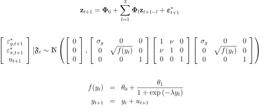
observable nonstationary factor. More specifically, we assume

F(yt) =



 

σg 0

0 pf(yt)



 ,

and follow Lee (2008) to make f(y) = θ0 + _{1+exp (}θ1_−λy), with θ0 > 0, θ1 > 0, λ > 0, yt+1 =

yt+ut+1, and

     

εg,t+1

επ,t+1

ut+1

     

|F_t∼iidN

            0 0 0       ,      

1 ν 0

ν 1 0

0 0 1             , (2)

where ε∗_t+1 = F(y_t)ε_t+1, with ε_t+1 = [ε_g,t+1, ε_π,t+1]′, F_t = σ({z_s}t_s=0) is the information

available at time t, and |ν| ≤1.

Under this stochastic volatility setup, we model volatility as a logistic function of a unit

root process, which implies that volatility is bounded and has a smooth transition between

two regimes: low volatility (θ0) and high volatility (θ0 +θ1), while the smoothness of the

transition is measured by the coefficientλ. Lee (2008) mentions this characteristic as opposed

to what happens with an exponential stochastic volatility model, in which volatility would

explode if there is enough persistence in it. Also, the smooth transition along with the

nonstationary latent factor {yt} allow for volatility clustering. Additionally, Park (2002)

shows that this type of nonlinear heteroscedasticity has sample kurtosis with truncated

supports. On a related matter, Kim et al. (2008) points out that since agents dislike the

uncertainty that arises when volatility is in between of the two regimes, because they would

The SV-VAR has some advantages with respect to other models used in the literature of

term structure of interest rates with recursive preferences and/or stochastic volatility. First,

we assume that the lag order of the VAR is finite, as opposed to the invertible VARMA(1,1)

proposed by PS. Second, we allow for the lag order of SV-VAR to be greater than one,

extending the setup in Boudoukh (1993).

2.3

Pricing bonds

In this section we use the intertemporal marginal rate of substitution to price bonds

under the SV-VAR specification for endowment growth and inflation rates. It is important

to point out that we do not make any assumption about the value of the EIS, as opposed to

PS, who set this coefficient to unity.

2.3.1 Real bond pricing

Recalling the pricing equation for bonds, we have that if the price, in consumption units,

att of a bond of maturity n is denoted by Qn,t, then

Qn,t=Et(Mt+1Qn−1,t+1) (3)

In equilibrium, the real pricing kernel is given by (1) with ct=et and Vt being the value of

utility. Consequently, the (log of the) pricing kernel in equilibrium is given by

lnMt+1 = lnβ+ (ρ−1)gt+1+ (α−ρ) (lnVt+1−lnµt(Vt+1)), (4)

where gt+1 ≡ ln(et+1/et) is the endowment growth rate between t and t+ 1. To obtain a

fully parametric (and able to be simulated) expression for the (log of the) pricing kernel, we

follow GHPZ. We obtain the following result, whose derivation appears in the Appendix:

where the approximation follows because of the linear approximation that we made to the

logistic function. At is an expression that includes preference parameters, parameters from

the SV-VAR and variables at t. v1, w1 and vf are parameters from the (log of the scaled)

value function which, in turn, are functions of the preference parameters and parameters from

the SV-VAR. Again, if α = ρ, we return to the conventional real pricing kernel obtained

from a power utility setup.

2.3.2 Nominal bond pricing

Since the pricing equation (3) must hold for real prices of nominal bonds, we have

Q$

n,t

Pt

=Et

Ã

Mt+1

Q$n−1,t+1

Pt+1

!

,

whereQ$

n,tdenotes the nominal price attof a bond maturingnperiods ahead, andPtdenotes

the price of the consumption good at t. Therefore, we can write

Q$_n,t=Et

¡

M_t$₊₁Q$_n−1,t+1¢

, (6)

where the (log of the) nominal pricing kernel is given by

lnM_t$₊₁ = lnMt+1−πt+1.

From the structures of the real and the nominal pricing kernels, we can see that the properties

of inflation influence the price of nominal bonds. Let us analyze the effects of inflation on

the real pricing kernel (5). First, under the power utility setup, the effect of inflation on

the pricing kernel is weighted by the EIS only (or the coefficient of relative risk aversion).

Second, under recursive preferences, inflation not only enters the pricing kernel weighted by

the EIS, but also by the difference between the coefficient of relative risk aversion and the

is determined by the difference between the coefficient of relative risk aversion and the EIS

too.

3

SV-VAR Estimation

In this section we proceed to estimate the parameters of the SV-VAR which will serve as

inputs for the estimation of preference parameters which, in turn, will allow us to simulate

the term structure of interest rates.

To estimate the model presented in section 2.2 we use annualized quarterly consumption

growth and inflation covering the period 1952:1 - 2008:3. We specify consumption as real

per capita consumption of nondurables and services as reported by the Bureau of Economic

Analysis. Data on the consumer price index (CPI) are from the Bureau of Labor Statistics

of the U.S. Department of Labor.

3.1

VAR lag selection and heteroscedasticity

In order to proceed with the estimation of the SV-VAR model we need to offer an adequate

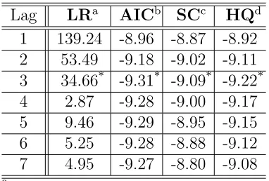
specification for the conditional mean vector of consumption growth and inflation. Table 1

reports values of four different lag order selection criteria of a homoscedastic VAR: Sequential

Modified LR, Akaike IC, Schwarz IC and Hannan-Quinn IC. The optimal lag order is 3,

according to all the criteria used. Additionally, with this lag order we do not reject the null

hypothesis of absence of serial correlation in the error term at the 1% level of significance.

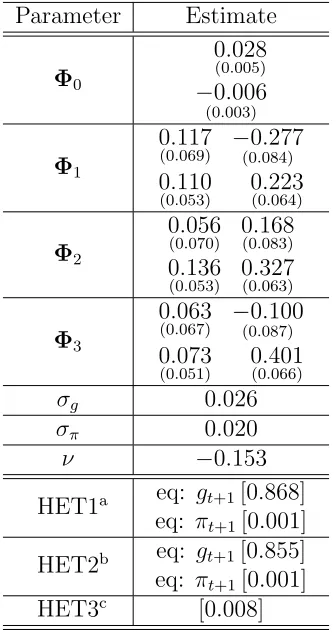
With the lag order set to 3 we proceed to estimate a homoscedastic VAR in order to

test for varying conditional variance. Table 2 shows results of the estimation as well as the

heteroscedasticity tests performed: ARCH LM test in each equation of the VAR,

single-equation White test, and joint White test. The first two tests reject the null hypothesis

of homoscedasticity in inflation but not in consumption growth at conventional significance

variance covariance matrix. All these results support our setup for the SV-VAR model with

respect to the assumption of including stochastic volatility in the inflation equation only.

3.2

Maximum likelihood estimation of the SV-VAR

We estimate parameters of the SV-VAR by maximum likelihood, using a nonlinear

Kalman filter to obtain the appropriate densities. Tanizaki (1996) shows how to construct

the prediction, updating and smoothing steps. First, notice that

zt+1|yt,Ft,Θ ∼ N

à Φ0+

3

X

l=1

Φlzt+1−l,Ω(yt)

!

(7)

yt|yt−1,Ft,Θ d

=yt|yt−1,Θ ∼ N(yt−1,1),

where Ω(yt) =F(yt)ΓF(yt), Θ is the parameter space, and Γ is the upper left 2×2 block of

the variance-covariance matrix in (2).

The maximum likelihood estimator is given by

ˆ

Θ = arg max

Θ

l(z₁, . . . ,z_n|Θ),

where l(z₁, . . . ,z_n|Θ) =

n

X

t=1

lnp(z_t|F_t−1,Θ), and

p(z_t|F_t−1,Θ) = Z

p(z_t, yt−1|Ft−1,Θ)dyt−1

= Z

p(z_t|yt−1,Ft−1,Θ)p(yt−1|Ft−1,Θ)dyt−1.

In order to integrate out the non observable and non stationary variableyt, we proceed to

numerically integrate the densities in which it appears. To that end, we apply the approach

used in Lee (2008) and described in extent in the Appendix along with details about the

prediction and updating steps of the filter. Results of the estimation are shown in Table 3.

are very similar to those obtained from the homoscedastic VAR(3) in Table 2. Regarding

parameters of the conditional volatility, all of them are statistically significant (positive) at

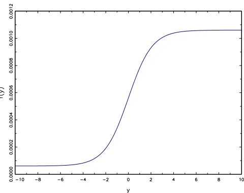
the 5% level of significance. In particular, given these estimates, the shape of the logistic

function is shown in Figure 1. The figure shows the smooth transition from the low volatility

regime to the high volatility one. The transition is determined by the parameter λ, which

is close to one, implying a transition smooth enough to make agents dislike a scenario of

moderate volatility because they do not know where the economy will end up, as mentioned

previously.

From the estimation of the SV-VAR, and by making use of a non linear Kalman filter,

we obtain the filtered volatility, which appears in Figure 2 along with the short rate and the

NBER recession periods. The graph shows that volatility is indeed highly persistent. It also

shows a highly volatile period between the second half of the 1970s and during the 1980s.

There is also a low volatility regime which corresponds to the period between the early 1990s

until the early 2000s. It is also evident an increase in volatility at the end of the present

decade due to the effects of the current crisis. In fact, volatility increases every time that a

recession affects the economy, except for one crisis episode at the beginning of the sample.

When comparing time series of the filtered volatility with those of the short-term nominal

interest rate, we can see that there is a positive covariation between them, except for the

period between the early 1990s and the mid 2000s. This is a sign that our volatility setup

could help capture salient features of interest rates 1 _{along with the other factors used here,}

namely, consumption growth and inflation.

4

Implications for bond yields

We describe the methodology for preference parameters estimation as well as comparisons

with results in other studies of equilibrium modeling of the term structure in Section 4.1. In

Section 4.2 we discuss the term structure implications of the model. In Section 4.3 we show

the model performance with respect to reproducing time series characteristics of the short

term yield and the yield spread. Here we use yields of maturities 1, 4, 8, 12, 20, 28 and 40

quarters. Data up to 1991 are from McCulloch and Kwon (1993), then we use yields on U.S.

Treasury securities at constant maturities reported by the Federal Reserve Bank.

4.1

Preference parameter estimation

Besides parameters involving preferences towards risk (α) and preferences towards

in-tertemporal allocations of consumption (ρ), we have additional parameters involved in the

(log of the) pricing kernel. The parameters under discussion include the discount factor, β,

and other parameters related to the (log of the scaled) value function, namely, v1, w1, and

vf, as well as other that appear inAtand that are related to the value function too (they are

denoted v2, v3, w2, andw3). Given α and ρ, these eight additional parameters are obtained

from a system of nonlinear equations designed to match the mean of the short-term interest

rate. The system of equations is shown in detail in the Appendix.

Regarding the preference parameters α and ρ, we estimate them so that the mean of

the yields produced by our model match as closely as possible the observed average term

structure. To that end, we make use of the simulated method of moments firstly introduced

by Lee and Ingram (1991), and extended by Burnside (1993) to the numerical solution to

asset pricing models proposed by Tauchen and Hussey (1991).

Before proceeding to the estimation of preference parameters we notice that, given the

nature of the logistic function assumed for volatility, we can define the process{ft+1}∞t=−∞≡

{f(yt+1)}∞t=−∞ with a well defined conditional density function,p(ft+1|ft), since the Markov

property of the process {yt}∞t=−∞ is inherited by {ft+1}∞t=−∞ because f(·) is bijective. We

show the expression for p(ft+1|ft) in the Appendix. This step is important because it allows

us to restrict the range of an integration from (−∞,∞) to an integration on (θ0, θ0 +θ1),

which is bounded.

is a function of z_t+1, ft+1, st, and ft, the nominal pricing kernel is also a function of these

variables. We write M$_(z

t+1, ft+1,st, ft) to express the dependence of the nominal pricing

kernel on the mentioned variables. Therefore, the pricing equation (6) implies that nominal

bond prices are functions of st and ft only:

Q$_n,t=Hn(st, ft),

with H0(st, ft) = 1 ∀t, and

Hn(st, ft) = EtM$(zt+1, ft+1,st, ft)Hn−1(st+1, ft+1) (8)

= Z ∞

−∞

Z θ0+θ1

θ0

M$(zt+1, ft+1,st, ft)Hn−1(st+1, ft+1)p(zt+1, ft+1|st, ft)dft+1dzt+1.

Further, we notice that the conditional density involved in the integration can be written as

follows:

p(zt+1, ft+1|st, ft) = p(zt+1|st, ft, ft+1)p(ft+1|st, ft)

= p(z_t+1|s_t, ft)p(ft+1|ft),

where passing from the first to the second identity is done becausezt+1|Ft, ft is independent

of ft+1, as shown in (7), and because {ft+1}∞t=−∞ is first-order Markov.

We also point out that there is an integration across three dimensions involved in (8).

Tauchen and Hussey (1991) suggests using a Gaussian quadrature method to discretize the

space of the state variables in order to write

Hn(sj, fl) = Nz

X

i=1

Nf

X

k=1

with

Πji,l = Prob{zt+1 =zi|st=sj, ft=fl}

Πlk = Prob{ft+1 =fk|ft =fl},

where j = 1,2, . . . ,Nzˆ ,l = 1,2, . . . , Nf, and ˆNz =Nz3. Here Nf and ˆNz denote the number

of quadrature abscissa points.2 _{We assume the same number of abscissa points for each of the}

variables in the VAR, which is 5, makingNz= 25 and ˆNz= 15,625. Furthermore, we assume

Nf = 6, making the total number of abscissa points ˆNz×Nf = 93,750. In the Appendix we

discuss the approach of Tauchen and Hussey to obtain the transition probabilities.

In order to obtain an extension from the discrete-space solution (9) to the

continuous-space solution, we use step functions. Burnside (1999) points out that any Gaussian

quadra-ture rule divides the real line for each of the variables into non-overlapping segments,

there-fore we can extend the discrete-space solution to any s ∈ R3 _{and f ∈ (θ0, θ0 +θ1). In the}

Appendix we discuss how to obtain this result.

Once we are able to obtain yields for different maturities from the model, we proceed to

estimate preference parameters by the simulated method of moments whose setup is shown

in the Appendix. For the moments we choose the means of yields, that is, we have 7 moment

conditions. Results of the estimation are shown in Table 4.

These results imply that the coefficient of relative risk aversion is approximately 4, while

the EIS is infinite. As mentioned before, β is estimated to match the average short-term

interest rate. The value of the coefficient of risk aversion is lower (and significantly lower in

some cases) compared to those obtained in the literature of term structure modeling with

recursive preferences. Values range from 5-7 in GHPZ, 16-17 in Doh (2008), and 43-85 in

PS. The value of the coefficient of EIS in this study is the same as the one obtained in

2_{Notice that the value for the abscissa points as well as the weights of the quadrature depend on the}

GHPZ, much higher than the unity coefficient assumed in PS, and the estimated coefficient

in Doh (2008), which is in the range 1.4-1.6. We notice that, since γ > 1

ψ, meaning that

agents prefer an early resolution of uncertainty, our volatility setup is compatible with the

preferences used in this study.

PS needs the risk aversion coefficient to be in the mentioned range because, given that

the EIS is set to unity, the only way to generate a positive expected excess return is by

giving an important weight to the negative covariance between inflation and expected future

consumption growth. The mechanism that allows PS and our work to have a positive excess

return has to do with the fact that higher inflation rates (that affect real payoffs of nominal

bonds, particularly long bonds) bring news about lower expected consumption growth rates

and, since the real payoff of long bonds is lower in bad times and agents prefer an early

resolution of uncertainty, the required premium on these bonds increases compared to short

bonds.

With respect to the EIS parameter, we point out that the higher it is, the less demand

for smoothing consumption over time. Increasing the EIS decreases the demand for

long-term real bonds to smooth consumption, leading to a higher required real premium on these

bonds. The fact that the EIS is high allows us to reproduce more satisfactorily the slope of

the term structure. Epstein and Zin (1991) mentions the infinite-elasticity case as the case

in which the C-CAPM reduces to the static CAPM, and points out that the static CAPM

emerges due to the perfect substitutability of consumption across time.

4.2

Term structure implications

We obtain time series for each of the yields with the same time horizon as the sample

data, 1952:1 to 2008:3, using the same step functions that allowed us to extend the

discrete-space solution to the continuous-discrete-space one. That is, we consider the consumption growth

rate, inflation rate and filtered volatility of a particular quarter and choose the yield for

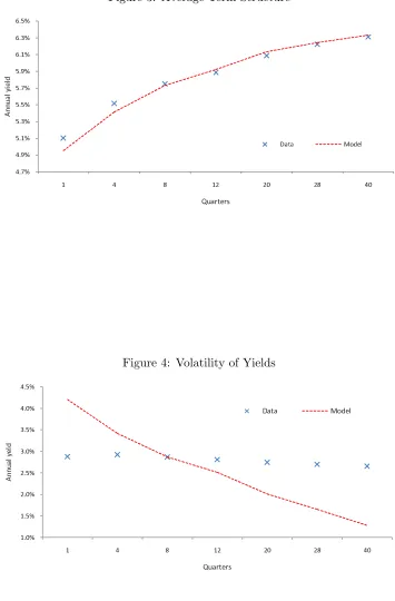
we show averages, standard deviations and first order autocorrelations of yields. The model

reproduces satisfactorily the average term structure but fails to reproduce the volatility of

yields. Particularly, the simulated yields’ volatilities decay in an exponential fashion with

respect to maturity, as opposed to the slowly decaying volatilities of observed yields. This

sharp decay is observed despite the introduction of a persistent factor for explaining yields,

which is the stochastic volatility. Figure 3 and Figure 4 show the average term structure and

the standard deviation of yields of both the observed and simulated data. The persistence of

the different yields, however, is satisfactorily reproduced by the model and here persistence

of the stochastic volatility process plays a fundamental role.

The reason for which the model is incapable of reproducing the slowly decaying

stan-dard errors of yields lies in the way the pricing equation (8) is computed. Here we use the

numerical integration technique suggested by Tauchen and Hussey (1991) and divided the

conditional density inside the integration into the product of two conditional densities: the

conditional density for the stationary processes, namely consumption growth and inflation,

and the conditional density for stochastic volatility, which is highly persistent. When

com-puting the numerical integral, we transform these densities into transition probabilities, and

the transition probabilities corresponding to consumption growth and inflation dominate the

transition probabilities for stochastic volatility, making the solution look like as if it came

from a purely stationary exogenous process. This situation can be more easily seen when

looking at equation (9), where the product of the two transition probabilities appears

explic-itly. Affine models of the term structure of interest rates under Epstein-Zin/Weil preferences

do not have this kind of problem because they can be solved explicitly by either assuming

that no correlation exists between consumption growth and inflation like in GHPZ, or by

4.3

Time series implications

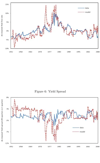
Figure 5 shows time series of the nominal yield on the three-month bond obtained from

the model and from observed data (both de-meaned). The simulated rate (dashed line) shows

more variability than the observed rate (solid line), but the model is able to satisfactorily

reproduce many of the movements in the short interest rate, except for a slight deviation

at the beginning of the 1990s and also at the end of the considered sample. The overall

correlation between the observed and the simulated rate is 0.73.

In Figure 6 we show the term spread of the 10-year bond with respect to the 3-month

bond. The simulated yield spread is more variable than the observed spread and the model

predicts a higher spread before the 1970s and a lower term spread during the 1970s than

what is observed. However, towards the end of the sample the model does a reasonable job

describing movements in the term spread. The overall correlation between the observed and

the simulated term spread is 0.14.

5

Conclusions

This paper presents an equilibrium model of the term structure of interest rates with

Epstein-Zin/Weil preferences and an exogenous process that includes logistic stochastic

volatility. The model’s performance is very reasonable with respect to matching the first

moment of the term structure of interest rates and the persistence of yields. The model,

however, is not good at reproducing the slowly decaying standard errors of yields with respect

to maturity. This last shortcoming occurs despite of the highly persistent stochastic

volatil-ity introduced as an additional factor to explain yields. The reason for the failure of the

model at explaining the standard deviation of yields lies in the way the numerical integration

to solve for the pricing equation is performed. Since the joint density inside the integration

can be split into the product of the conditional density for the stationary processes, namely

of the two is dominated by the first stationary conditional density, regardless of volatility’s

persistence.

The estimated preference parameters imply an infinite elasticity of substitution between

present and future consumption, whereas the coefficient of relative risk aversion toward static

lotteries is about 4. These estimates can be seen as an argument in favor of our volatility

specification (given that γ > _ψ1), since agents prefer an early resolution of uncertainty and our volatility function does not reveal the ending state if the initial volatility state is of

medium uncertainty.

One future line of research is to consider a semi-affine specification for the pricing kernel,

in the line of Duarte (2004), which is a flexible form that would allow us to incorporate

the covariance between consumption growth and inflation and, at the same time, avoid a

numerical integration to price bonds.

Another future line of research is to incorporate specifications of monetary or fiscal policy

6

Appendix

6.1

Derivation of the pricing kernel

In order to obtain equation (5), we need to make a linear approximation of the logistic function around some value ¯f ∈(θ0, θ0+θ1). We obtain

f(yt+1)≈f(yt) + ¯θut+1,

where ¯θ= λ(f¯_θ−₁θ0) ¡

θ0+θ1−f¯

¢

> 0. Also

p

f(yt)≈

1 2

à q

¯

f+ fp(yt) ¯

f

!

.

From here on, we follow Gallmeyer et al. (2007) in the derivations. By homogeneity of

µt(·) we can write

Vt

et

= ·

(1−β) +βµt

µ

Vt+1

et+1

× et+1

et

¶ρ¸1_ρ

.

Taking logs and defining vt= ln (Vt/et), we have

vt=

1

ρln [(1−β) +βexp (ρµ˜t)],

where ˜µt ≡ln (µt(exp (vt+1+gt+1))).

Approximating vt around ˜µt= ¯m yields

vt≈η0+η1µ˜t,

where

η0 =

1

ρln [(1−β) +βexp (ρm¯)]−

βexp (ρm¯)

1−β+βexp (ρm¯)m¯,

η1 =

βexp (ρm¯)

1−β+βexp (ρm¯), 0< η1 <1.

If we evaluate at ¯m= 0, these expressions imply η0 = 0, η1 =β.

In order to parameterize the log of the value function, conjecture that

which implies that

vt+1+gt+1 = ¯v+ (1 +v1)gt+1+v2gt+v3gt−1+w1πt+1+w2πt+w3πt−1+vff(yt+1) ≈ ¯v+ (1 +v1)gt+1+v2gt+v3gt−1+w1πt+1+w2πt+w3πt−1+ (11)

+vf

¡

f(yt) + ¯θut+1

¢

.

Taking conditional expectation and variance on (11), we obtain

Et(vt+1+gt+1) ≈ ¯v+ (1 +v1)Etgt+1+v2gt+v3gt−1 +w1Etπt+1+w2πt+w3πt−1+vff(yt),

vart(vt+1+gt+1) ≈ (1 +v1)2σg2+w12f(yt) + 2 (1 +v1)w1νσg

p

f(yt) +vf2θ¯2

≈ (1 +v1)2σg2+w12f(yt) + (1 +v1)w1νσg

à q

¯

f +fp(yt) ¯

f

!

+v_f2θ¯2

= (1 +v1)2σg2+

Ã

w2₁+ (1 +vp1)w_¯1νσg

f

!

f(yt) + (1 +v1)w1νσg

q ¯

f+v_f2θ¯2.

Since vt+1+gt+1 is normally distributed conditional on the information available att, we

have

˜

µt=Et(vt+1+gt+1) +

α

2vart(vt+1+gt+1), then

˜

µt ≈ v¯+ (1 +v1) Φ01+w1Φ02+

α

2 ·

(1 +v1)2σ2g+ (1 +v1)w1νσg

q ¯

f +v2_fθ¯2

¸ +

+h(1 +v1) Φ(1)11 +v2 +w1Φ(1)21

i

gt+

+h(1 +v1) Φ(2)11 +v3 +w1Φ(2)21

i

gt−1+

+h(1 +v1) Φ(3)11 +w1Φ(3)21

i

gt−2+

+h(1 +v1) Φ(1)12 +w1Φ(1)22 +w2

i

πt+

+h(1 +v1) Φ(2)12 +w1Φ(2)22 +w3

i

πt−1 +

+h(1 +v1) Φ(3)12 +w1Φ(3)22

i

πt−2+

+ "

vf +

α

2 Ã

w2₁+ (1 +vp1)_¯w1νσg

f

!#

f(yt),

where Φ(_ijl) is the element (i, j) ofΦl fori= 0,1,2, j = 1,2, andl = 0,1,2,3. Now, by using

vt ≈η0+η1µ˜t, (10), and η0 = 0, η1 =β, we can get ¯v, v1, v2,v3, w1, w2,w3.

Recall that

˜

µt ≈ v¯+ (1 +v1)Etgt+1+v2gt+v3gt−1+w1Etπt+1+w2πt+w3πt−1+vff(yt) +

+α 2

h

(1 +v1)2σg2+w21f(yt) + 2 (1 +v1)w1νσg

p

f(yt) +vf2θ¯2

i

and

lnVt+1−lnµt(Vt+1) =vt+1+gt+1−µ˜t,

therefore we have

lnVt+1−lnµt(Vt+1) ≈ (1 +v1) (gt+1−Etgt+1) +w1(πt+1−Etπt+1) +vf(f(yt+1)−f(yt))−

−α

2 h

(1 +v1)2σg2+w12f(yt) + 2 (1 +v1)w1νσg

p

f(yt) +v2fθ¯2

i

. (12)

Replacing (12) into (4) we obtain the real pricing kernel

lnMt+1 ≈ lnβ−(α−ρ)At+ [(ρ−1) + (α−ρ) (1 +v1)]gt+1+ (α−ρ) [w1πt+1+vff(yt+1)],

where

At = (1 +v1)Etgt+1+w1Etπt+1+vff(yt) +

+α 2

h

(1 +v1)2σ2g+w12f(yt) + 2 (1 +v1)w1νσg

p

f(yt) +vf2θ¯2

i

,

To obtain the nominal short-term interest rate, we need to get expressions forEt(lnMt+1−

πt+1) andvart(lnMt+1−πt+1) which, by the log-normality of the pricing kernel, allow us to

write

r$

t+1 ≈ −lnβ+ (1−ρ)Etgt+1+Etπt+1−

−1

2{σ˜

2

t −(α−ρ)α[(1 +v1)2σg2+w21f(yt) + 2(1 +v1)w1νσg

p

f(yt) +vf2θ¯2]},

where

˜

σ_t2 = [(ρ−1) + (α−ρ) (1 +v1)]2σ2g+ [(α−ρ)w1 −1]2f(yt) + (α−ρ)2vf2θ˜2+

+2 [(ρ−1) + (α−ρ) (1 +v1)] [(α−ρ)w1−1]νσg

p

f(yt).

6.2

Filtering procedure for the SV-VAR estimation

For the prediction step, we have3

p(yt|Ft,Θ) =

Z

p(yt, yt−1|Ft,Θ)dyt−1

= Z

p(yt|yt−1,Ft,Θ)p(yt−1|Ft,Θ)|, dyt−1

= Z

p(yt|yt−1,Θ)p(yt−1|Ft,Θ)dyt−1.

3_{Notice that, due to the nature of how the information is revealed,}

p(yt|Ft) refers to the density of

the prediction, whilep(yt|Ft+1) is the density for the updating step, oncezt+1 (and its variance) has been

For the updating step, we have

p(yt|Ft+1,Θ) = p(yt|zt+1,Ft,Θ)

= p(yt,zt+1|Ft,Θ)

p(z_t+1|F_t,Θ)

= p(zt+1|yt,Ft,Θ)p(yt|Ft,Θ)

p(zt+1|Ft,Θ)

.

Regarding the estimation strategy, we need to numerically integrate the densities in order to proceed to the maximization of the log-likelihood function. However, since the state variable may show high persistence, we will follow Lee (2008) to make the Gauss-Legendre quadrature rule depend on the previous value of the state. For the prediction step, we assume that p(yt−1|Ft) is being integrated over [−c+yt−1|t−1, c+yt−1|t−1] for some c > 0,

where yt−1|t−1 ≡E(yt−1|Ft−1) is the prediction ofyt−1. Then we have,

p(yt|Ft) =

Z

p(yt|yt−1)p(yt−1|Ft)dyt−1

≈

Z c+yt−1|t−1 −c+yt−1|t−1

p(yt|yt−1)p(yt−1|Ft)dyt−1

for t= 1, ..., n, with y0|1 to be estimated, andp(y0|F1) = 1 at y0|F1 =y0|1.

For the updating step we need p(zt+1|Ft), which can be approximated as follows:

p(zt+1|Ft) =

Z

p(zt+1|yt,Ft)p(yt|Ft)dyt

= Z Z

p(zt+1|ytFt)p(yt|yt−1)p(yt−1|Ft)dyt−1dyt

≈

Z c+yt|t

−c+yt|t

Z c+yt−1|t−1 −c+yt−1|t−1

p(zt+1|ytFt)p(yt|yt−1)p(yt−1|Ft)dyt−1dyt,

where yt|t =yt−1|t is the prediction of yt conditional on Ft. Now,

yt|t+1 ≈

Z c+yt|t

−c+yt|t

ytp(yt|Ft+1)dyt,

with p(yt|Ft+1) = p(zt+1|yt,

Ft)p(yt|Ft)

p(zt+1|Ft) .

We obtain the filtered stochastic volatility from

ft|t=

Z c+y_t|t

−c+yt|t

6.3

Nonlinear system of equations

The nonlinear system of equations is given by

v1 =

β

1−βΦ(1)gg

h

Φ(1)₁₁ +v2+w1Φ(1)21

i

v2 = β

h

(1 +v1) Φ(2)11 +v3+w1Φ(2)21

i

v3 = β

h

(1 +v1) Φ(3)11 +w1Φ(3)21

i

w1 =

β

1−βΦ(1)₂₂ h

(1 +v1) Φ(1)12 +w2

i

w2 = β

h

(1 +v1) Φ(2)12 +w1Φ(2)22 +w3

i

w3 = β

h

(1 +v1) Φ(3)12 +w1Φ(3)22

i

vf =

β

1−β α

2 Ã

w₁2+(1 +vp1)_¯w1νσg

f

!

¯

r$ _{= −lnβ+ (1−ρ)}h_Φ 01+

³

Φ(1)₁₁ + Φ(2)₁₁ + Φ(3)₁₁´¯g+³Φ(1)₁₂ + Φ(2)₁₂ + Φ(3)₁₂´π¯i+

+Φ02+

³

Φ(1)₂₁ + Φ(2)₂₁ + Φ(3)₂₁´¯g+³Φ(1)₂₂ + Φ(2)₂₂ + Φ(3)₂₂´π¯−

−1 2     

[(ρ−1) + (α−ρ) (1 +v1)]2σ2g+ [(α−ρ)w1−1]2f¯+ (α−ρ)2v2fθ¯2+

+2 [(ρ−1) + (α−ρ) (1 +v1)] [(α−ρ)w1−1]νσg

p ¯

f− −(α−ρ)αh(1 +v1)2σg2+w12f¯+ 2 (1 +v1)w1νσg

p ¯

f +v2

fθ¯2

i ,     

where ¯r$_{, ¯gand ¯πare the sample means of the short-term nominal interest rate, consumption}

growth and inflation, respectively. For ¯f we take the median of the filtered {ft} because of

the existence of the two specified volatility regimes.

6.4

Stochastic volatility’s transition density

The transition density for the stochastic volatility process is given by

p(ft+1|ft) =

     1 √ 2πλ ³ 1

ft+1−θ0 +

1

θ1+θ0−ft+1

´ exp

Ã

−₂1_λ2

µ ln

ft+1−θ0

θ₁₊θ₀−_ft+1

ft−θ0

θ1+θ0−ft

¶2!

if θ0 < ft+1 < θ0+θ1

0 o.w.

6.5

Transition probabilities

Assume that integration is performed against the densityp(zt+1|st, ft)p(ft+1|ft). Tauchen

the states for the stochastic volatility, the normalization is performed as follows:

Πji,l =

p(zi|sj, fl)

p(z_i|µs, fl) wz

i,l

az

j,l

,

Πlk =

p(fk|fl)

af_l w

f k, where az j,l = Nz X i=1

p(zi|sj, fl)

p(zi|µs, fl)

wz

i,l,

af_l =

Nf

X

k=1

p(fk|fl)wf_k,

wz

i,l, for i= 1,2, . . . , Nz, denote the weights given by the Gauss-Hermite quadrature;w f k, for

k = 1,2, . . . , Nf, denote the weights given by the Gauss-Lebesgue quadrature, and µs is the

unconditional mean of {z_t}∞

t=−∞.

6.6

Continuous-space solution from discrete-space solution

We can extend the discrete-space solution to the continuous-space solution by letting

Hn(s, f) =

ˆ Nz X j=1 Nf X l=1

Hn(sj, fl)1j,l(s)1l(f),

where 1_{j,l(s) =}1_l(z1)1_l(z2)1_{l(z3), and}

1_{l(zi) =}

(

1, if z_i ∈(xz

j−1,l,x

z

j,l)

0, otherwise,

1_{l(f) =}

(

1, if f ∈(xf_l−1, xf_l) 0, otherwise,

with xz

j,l = µz+ chol(Ω(fl))xj,l, where xj,l is the solution to wj,lz =

Rx_j,l

x_j−1,lexp (−v

′_v)dv,

x_0,l =−∞,x_Nz,l =∞, andwz

j,l are the weights given by the Gauss-Hermite quadrature rule.

In a similar reasoning, xf_l = xf_l−1+ 1₂θ1wfl, where x f

0 = θ0, xfNf = θ0+θ1, and w

f

l are the

weights given by the Gauss-Lebesgue quadrature rule.

6.7

Simulated method of moments estimation

The estimators are defined, for Υ ≡ {(−∞,1),(−∞,1)}, as

{α,ˆ ρˆ}= arg min

{α,ρ}∈Υ

where, forr_t denoting the vector of yields for the different maturities considered,

mT(α, ρ) =

1

T

T

X

t=1

ψ(rt, α0, ρ0)−µT(α, ρ),

and α0 and ρ0 are the true preference parameters. For the estimation we choose the means

of the yields, which give us 8 moment conditions, that is, we choose ψ(·) to be the identity function. For DT we use the inverse of a HAC variance-covariance matrix of the method of

References

Backus, D., and S.E. Zin (1994) ‘Reverse engineering the yield curve.’NBER Working Paper No. 4676

Backus, D.K., A.W. Gregory, and S.E. Zin (1989) ‘Risk premiums in the term structure: Evidence from artificial economies.’ Journal of Monetary Economics24(3), 371–99

Boudoukh, J. (1993) ‘An equilibrium model of nominal bond prices with inflation-output correlation and stochastic volatility.’Journal of Money, Credit and Banking25(3), 636–65

Burnside, C. (1993) ‘Consistency of a method of moments estimator based on numerical solutions to asset pricing models.’ Econometric Theory 9(4), 602–32

(1999) ‘Discrete state-space methods for the study of dynamic economies.’Computational Methods for the Study of Dynamic Economies (Oxford University Press, New York, NY)

Campbell, J.Y., and R.J. Shiller (1991) ‘Yield spreads and interest rate movements: A bird’s eye view.’Review of Economic Studies 58(3), 495–514

Canova, F., and J. Marrinan (1996) ‘Reconciling the term structure of interest rates with the consumption-based ICAP model.’Journal of Economic Dynamics and Control20(4), 709– 50

Doh, T. (2008) ‘Long Run Risks in the Term Structure of Interest Rates: Estimation.’ The Federal Bank of Kansas City RWP 08-11

Donaldson, J.B., T. Johnsen, and R. Mehra (1990) ‘On the term structure of interest rates.’

Journal of Economic Dynamics and Control 14(3), 571–96

Duarte, J. (2004) ‘Evaluating an alternative risk preference in affine term structure models.’

Review of Financial Studies 17(2), 379–404

Epstein, L.G., and S.E. Zin (1989) ‘Substitution, risk aversion, and the temporal behavior of consumption and asset returns: A theoretical framework.’ Econometrica 57(4), 937–69

(1991) ‘Substitution, risk aversion, and the temporal behavior of consumption and asset returns: An empirical analysis.’ The Journal of Political Economy99(2), 263–86

Gallmeyer, M.F., B. Hollifield, F. Palomino, and S.E. Zin (2007) ‘Arbitrage free bond pric-ing with dynamic macroeconomic models.’ The Federal Reserve Bank of St Louis Review

89(4), 305–26

Kim, H., H.I. Lee, J.Y. Park, and H. Yeo (2008) ‘Macroeconomic Uncertainty and Asset Prices: A Stochastic Volatility Model.’ Technical Report, Working Paper

Lee, H.I. (2008) ‘Stochastic volatility models with persistent latent factors: theory and its applications to asset prices.’ PhD dissertation, Texas A&M University

McCulloch, J.H., and H.C. Kwon (1993) ‘US term structure data, 1947-1991.’ Technical Report, Working Paper No. 93-6, The Ohio State University

Park, J.Y. (2002) ‘Nonstationary nonlinear heteroskedasticity.’ Journal of econometrics

110(2), 383–415

Pennacchi, G.G. (1991) ‘Identifying the dynamics of real interest rates and inflation: Evi-dence using survey data.’The review of financial studies 4(1), 53–86

Piazzesi, M., and M. Schneider (2006) ‘Equilibrium yield curves.’ NBER Macroeconomics Annual 21(1), 389–42

Tanizaki, H. (1996) Nonlinear filters: estimation and applications(Springer Verlag)

Tauchen, G., and R. Hussey (1991) ‘Quadrature-based methods for obtaining approximate solutions to nonlinear asset pricing models.’Econometrica 59(2), 371–96

Wachter, J.A. (2006) ‘A consumption-based model of the term structure of interest rates.’

Table 1: Lag order selection of the VAR

Lag LRa AICb SCc HQd 1 139.24 -8.96 -8.87 -8.92 2 53.49 -9.18 -9.02 -9.11 3 34.66* _-9.31* _-9.09* _-9.22*

4 2.87 -9.28 -9.00 -9.17 5 9.46 -9.29 -8.95 -9.15 6 5.25 -9.28 -8.88 -9.12 7 4.95 -9.27 -8.80 -9.08

a_{Sequential modified LR test statistic.}

b

Akaike information criterion.

c

Schwarz information criterion.

d_{Hannan-Quinn information criterion.} *

Lag order selected by the criterion.

Table 2: Consumption Growth and Inflation VAR

Parameter Estimate

Φ0

0.028

(0.005) −0.006

(0.003)

Φ1

0.117

(0.069) −(00..084)277

0.110

(0.053) 0(0..223064)

Φ2

0.056

(0.070) 0(0..168083)

0.136

(0.053) 0(0..327063)

Φ3

0.063

(0.067) −(00..087)100

0.073

(0.051) 0(0..401066)

σg 0.026

σπ 0.020

ν −0.153

HET1a eq: gt+1[0.868]

eq: πt+1[0.001]

HET2b eq: gt+1[0.855]

eq: πt+1[0.001]

HET3c _[0.008]

Values in parenthesis denote standard errors. Values in square brakets denote p-values.

a

ARCH LM test.

b

White heteroskedasticity test with cross terms for individual equations.

c_{Joint White heteroskedasticity test with cross}

terms.

z_t+1 =Φ₀ +

3

X

l=1

Φ_lz_t+1−l+ε_t+1

·

εg,t+1

επ,t+1

¸

|F_t∼iidN

µ· 0 0

¸

,

·

σg 0

0 σπ

¸ · 1 ν ν 1

¸ ·

σg 0

0 σπ

Table 3: Estimates of the SV-VAR

Parameter Estimate

Φ0

0.030

(0.004) −0.007

(0.002)

Φ1

0.108

(0.067) −(00..082)302

0.105

(0.040) 0(0..186069)

Φ2

0.050

(0.068) 0(0..158083)

0.123

(0.042) 0(0..356068)

Φ3

0.066

(0.066) −(00..085)078

0.089

(0.039) 0(0..402065)

σg 0.026

(0.001)

θ0 6.05×10−5 (2.15×10−5₎

θ1 0.001 (3.6×10−4₎

λ 0.950

(0.403)

ν −0.175

(0.067)

Values in parenthesis denote standard errors.

z_t+1 =Φ₀ +

3

X

l=1

Φ_lz_t+1−l+ε∗_t+1

  ε∗ g,t+1 ε∗ π,t+1

ut+1



|F_t∼N     0 0 0  ,  

σg 0 0

0 pf(yt) 0

0 0 1



 



1 ν 0

ν 1 0 0 0 1



 



σg 0 0

0 pf(yt) 0

0 0 1



 



f(yt) = θ0+

θ1

1 + exp (−λyt)

Table 4: Estimates of α,

ρ, and β

Parameter Estimate

α −3.014

(0.050)

ρ 0.999

(0.016)

β 0.982

Values in parenthesis denote standard errors.

βcomes from the solution to the non-linear system of equations.

Table 5: Moments of the Yield Curve

E(y1

t) E(yt4) E(yt8) E(y12t ) E(yt20) E(yt28) E(y40t )

data 5.100 5.514 5.748 5.885 6.085 6.222 6.311

model 4.953 5.412 5.731 5.922 6.133 6.242 6.332

σ(y1

t) σ(yt4) σ(yt8) σ(yt12) σ(yt20) σ(y28t ) σ(yt40)

data 2.877 2.922 2.866 2.812 2.743 2.700 2.653

model 4.203 3.414 2.868 2.512 2.007 1.649 1.279

ρ(y1

t, y1t−1) ρ(yt4, y4t−1) ρ(yt8, y8t−1) ρ(yt12, yt12−1) ρ(y20t , yt20−1) ρ(yt28, yt28−1) ρ(yt40, y40t−1)

data 0.926 0.935 0.942 0.948 0.958 0.963 0.968

model 0.882 0.912 0.922 0.925 0.927 0.927 0.927

Numbers are annual percentages, except for autocorrelations.

Figure 1: Implied Logistic Function

Figure 2: Filtered Logistic Volatility

Figure 3: Average Term Structure

✁✂ ✄ ✁☎ ✄ ✆ ✁✝ ✄ ✆ ✁✞ ✄ ✆ ✁✆ ✄ ✆ ✁✂ ✄ ✆ ✁☎ ✄ ✟ ✁✝ ✄ ✟ ✁✞ ✄ ✟ ✁✆ ✄

✝ ✠ ✝✡ ✡ ☛ ✡✠ ☛

☞✌

✌

✍✎

✏

✑

✒✓

✏✔

✕ ✖✗ ✘ ✙✚✘✛

✜ ✢ ✣✢

✤✥✦✧★

Figure 4: Volatility of Yields

✁✂ ✄ ✁☎ ✄ ✆ ✁✂ ✄ ✆ ✁☎ ✄ ✝ ✁✂ ✄ ✝ ✁☎ ✄ ✞ ✁✂ ✄ ✞ ✁☎ ✄

✞ ✟ ✆ ✆✂ ✆ ✟ ✞ ✂

✠✡

✡

☛☞

✌

✍✎

✌✏

✑ ✒✓ ✔✕ ✖✔✗

✘

✓ ✕ ✓ ✙✚

✛ ✖

Figure 5: Risk-free Rate ✁ ✂ ✄ ☎ ✄ ✂ ✄ ☎ ✄ ✁ ✂ ✄ ✁ ☎ ✄ ✁ ✆☎ ✝ ✁ ✆☎ ✞ ✁ ✆✟ ✠ ✁ ✆✡ ✂ ✁ ✆✡ ✡ ✁ ✆✞ ☛ ✁ ✆✞ ✆ ✁ ✆✆ ☎ ✝ ✂✂ ✝ ✝ ✂✂ ✞ ☞✌ ✍ ✎✌ ✏✑ ✌ ☞ ✒✓✔ ✕ ✍ ✖✗ ✌ ✌ ✗ ✏ ✘✌ ✙ ✚ ✛✚ ✜✢ ✙ ✣ ✤

Figure 6: Yield Spread