An Influence of the Noise on the Imaging Algorithm
in the Electrical Impedance Tomography
*
Hui Zhang1, Li Wang1, Yongjun Zhou1, Peijie Zhang2, Jixia Wu1, Ying Li3
1Faculty of Physics and Electronic Engineering, Xianyang Normal University, Xianyang, China 2School of Highway, Chang’an University, Xi’an, China
3Department of Civil, Environmental and Geomatic Engineering, University College London, London, UK
Email: [email protected]
Received July 24,2013; revised August 31, 2013; accepted September 16, 2013
Copyright © 2013 Hui Zhang et al. This is an open access article distributed under the Creative Commons Attribution License, which permits unrestricted use, distribution, and reproduction in any medium, provided the original work is properly cited.
ABSTRACT
Electrical impedance tomography (EIT) reconstructs the internal impedance distribution of the body from electrical measurements on body surface. The algorithm research is one of the main problems of the EIT. This paper presents the MPSO-MNR Algorithm, which is formed by combining the Modified Particle Swarm Optimization (MPSO) with Modified Newton-Raphson algorithm (MNR), gives the reconstruction results of certain configurations and analyzes the influence of the noise on the MPSO-MNR algorithm in the EIT. The numerical results show that the MPSO-MNR algo-rithm can reconstruct the resistivity distribution within the certain iterations. With the moving of the target to the centre of 2-D solution domain and the increase of noise, the border of the reconstruction objects becomes vague, and the fit-ness value and the total error increase gradually.
Keywords: MPSO-MNR Algorithm; Signal-To-Noise Ratio; Objective Function; EIT
1. Introduction
Electrical impedance tomography (EIT) is a non-invasive imaging technique, which aims to reconstruct images of internal electrical property (conductivity, permittivity and permeability in some high-frequency non-medical applications) distributions and variations by making elec-trical measurements on the body’s surface [1]. The im-aging methods are classified as dynamic or static imag-ing form. The static imagimag-ing method reconstructs the electrical parameter distribution in the solution domain. Static EIT imaging problem is solved by transforming the problem into an objective function, and using the iterative method to achieve the electrical parameter re-construction [2,3], because it is the nonlinear inverse problem.
Algorithm research is one of the main problems of the static EIT. Based on deterministic and stochastic opti-mizers, many static EIT algorithms have been proposed [2,3], such as Modified Newton-Raphson (MNR) algo-rithm [4], Double Constraint Method (DCM), Layer Stripping Method (LSM), the reconstruction algorithms
based on the Particle Swarm Optimization (PSO) [5-7], Genetic algorithm (GA) [8] etc. In recent years, some synthetic algorithms have been proposed, for example, Homotopy-Modified Newton-Raphson algorithm (H- MNR) [1], and MPSO-MNR algorithm [9]. From a com- putational point-of-view, the deterministic techniques (e.g., MNR methods) are very attractive, for example, MNR algorithm has the fast convergence speed and the calibration nature. However, the starting trial solution should be closed enough to the “actual” solution. The use of the stochastic genetic algorithms (GA) would, in prin-ciple, avoid such a circumstance. But in the GA, various numerical parameters must be carefully calibrated and customized to the application. PSO is a robust stochastic algorithm which overcomes GA’s drawbacks [10]. Tak-ing into account the features of PSO and MNR, we com-bine the advantages of MPSO and MNR algorithm to form the MPSO-MNR algorithm. Its performance and influence of the noise on the PSO-MNR are analyzed and discussed in this paper.
The paper is structured as follows. After the introduc-tion of the mathematical model of the EIT (Secintroduc-tion 2), Section 3 presents the MPSO-MNR algorithm, Section 4 presents a case study to show the MPSO-MNR algorithm
performance and the influence of the noise on the recon-struction results. Section 5 provides some concluding re- marks.
2. Mathematical Model
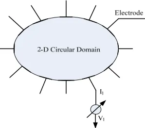
The principle of operation of EIT is shown in Figure 1, where the electrical current is injected according to the certain driven pattern, and the electrical potential of the body’s surface is measured by the electrodes. Based on electromagnetic theory, when an injected electrical cur-rent is at a sufficiently low frequency, the EIT problem can be treated as a quasi-static problem. Given the resis-tivity distribution inside the body, the potential satis-fies the Laplace’s equation and the boundary conditions as follows [11]:
1
0
in solution domain, (1)
l
z n
l
at measuring electrodes, (2)
1
l
J n
at the current injection electrodes, (3)
1 0
n
at no-injection electrodes. (4)
where is the electrical resistivity distribution in 2-D circular domain , l is the contact impedance on l-th
electrode, l
z
J is the electric current density at l-th elec-
trode respectively, L is the total electrode numbers. In this paper, we subdivided the 2-D circular solution domain into small cells by using Finite Element Method (FEM) (see Figure 2).
[image:2.595.351.497.84.247.2]The EIT problem is an ill-posed inverse problem. Given the electrical resistivity distribution in the solution domain and the injected current at the body’s surface, the forward problem of the EIT is to solve the potential dis- tribution in the solution space. The inverse problem is to reconstruct the resistivity distribution by the measuring electrical potential at the electrodes.
Figure 1. Principle of operation of EIT.
−1 −0.5 0 0.5 1 1
0.5
0
−0.5
[image:2.595.98.247.587.719.2]−1
Figure 2. 2-D circular model.
For the all-electrode current model, the EIT problem can be written as [11]:
1 ,
bA I (5)
where, N L1
bR
b
, the elements from 1 to of the matrix are the electrical potential of all FEM node in solution domain, and from to are the electrode potential. L
N
1
1
N
1, ,2NL
TI I I I is the vector of
the injecting electrical current. The matrix A consists
of the stiffness matrix of FEM and the coefficient matrix of the electrodes.
The iterative method is used to reconstruct the resistiv-ity distribution. Given the initial value of the MPSO- MNR algorithm at random, to update constantly the re-sistivity distribution by comparing the changes of the fitness value and the total error until the end condition is satisfied.
3. MPSO-MNR Algorithm
PSO has been shown to be effective in optimizing diffi-cult multidimensional discontinuous problems in a vari-ety of fields, it is not rigorous demand for the iterative initial value. MNR has the high computational efficiency when the starting trial solution is closed to the true value. In view of the advantages of the PSO and MNR algo-rithm, the MPSO-MNR algorithm is formed in EIT. The idea of the MPSO-MNR is to produce an initial value closed to the true value by MPSO, to acquire the resistiv-ity distribution through MNR algorithm.
3.1. Modified Particle Swarm Optimization
[6,7,10].
In this paper, MPSO updates the population using the population mutation method, which is to update some particles using (6), and the other particles track the per-sonal best and global best by using (7), (8),
1 0 5 0 5
k
i ig
x . * P . * rrp* rand, (6)
1
1 1 2 2
k k k k k
i i ib i ig
v wv c r p x c r p xk
i
1
, (7)
1
k k k
i i i
x x v , (8)
where is dynamic inertia weight, is the maxi-mum empirical value of the electrical resistivity in solu-tion domain, rand is the random number between 0
and 1.
w rrp
Definition: Fitness Value Function Ff:
1 1l es t
l l
i
f L t
l l
v v F
v
ρ . (9)
3.2. MNR Algorithm
Definition: Objective Function f :
2
0 2 0
1 1
2 2
T
f ρ v ρ v v ρ v v ρ v0
k
,(10)
where is the vector of the electrical resistivity distri-bution, 0, are the measuring and the
calcula-tion electrical potential value at the surface electrode, respectively. The -th iteration of using MNR algorithm is
ρ
v v
ρ1
k ρ
k1 k Δ
ρ ρ ρ , (11) where
1
0
Δ k k T k k T v k v
J J J
ρ ρ ρ ρ ρ
, (12)
i
ij j
J
ρ v ρ (13)
is the Jacobian matrix.
3.3. MPSO-MNR Algorithm Flow [9]
1) Set up the FEM model in the solution space.
2) Obtain the initial value of the MNR by the MPSO algorithm.
Step a). Initialization. Initialize the particle position , velocity , Set the acceleration constant , and inertia constant .
0
ρ v0
1 c c2
w
Step b). Calculate and evaluate the particle’s fitness value, compare and obtain the ib, ig.
Step c). Calculate the particle’s velocity, update the swarm.
P P
Step d). Repeat.
3) Reconstruct by the MNR algorithm.
Step a). Using the numerical result of the MPSO algo-rithm as the initial value 0
ρ , to calculate the objective
function value 0 f ρ .
Step b). If the end condition is met, end iteration, else go to step c).
Step c). Calculate objective function f
ρk1 k
. Step d). Calculate k1 k Δ ,
ρ ρ ρ k k 1, go to step b).
4. Numerical Simulation
Definition: Total Error (TE)1
1
m es t
i i
i
m t
i i
TE
(14)where es i
and t i
are the reconstruction value and the true value of the resistivity in the solution domain, re-spectively. is the element numbers of the solution domain.
m
Definition: Signal-to-Noise Ratio (SNR)
0
20log
SNR v l n , (15)
where v l0
is the measure potential value at the -th,is the sampling noise amplitude.
l
n
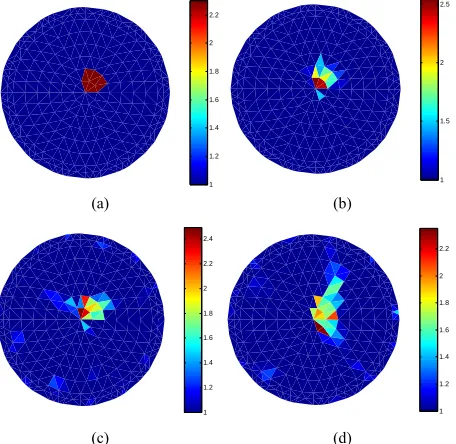
4.1. Single Target Simulation
A simulation target is set in the 2-D circular domain (see
Figures 3(a) and 4(a)), the background resistivity is 1
Ω·m, the target is 2.3 Ω·m. The iterative initial value of the MPSO algorithm is set as the random value between 1 and the empiric value. According to the trend of the fitness value and the total error with the number of itera-tions, the economic iterations of the MPSO should be about 10 times, MNR algorithm about 20 times [9]. In order to compare the reconstruction results in different configurations and noise levels, the 50-th iteration results of the MPSO is serve as the iterative initial value of the MNR algorithm, the end condition of the MPSO-MNR algorithm is at 60-th times of the MNR iteration in this paper.
1 1.2 1.4 1.6 1.8 2 2.2
1 1.2 1.4 1.6 1.8 2 2.2 2.4
(a) (b)
1 1.5 2 2.5
1 1.2 1.4 1.6 1.8 2 2.2 2.4 2.6 2.8
[image:4.595.58.291.82.308.2](c) (d)
Figure 3. Simulation model and the reconstruction result of the single target. (a) Simulation target; (b) Reconstruction result (non-noise); (c) Reconstruction result (SNR = 40 dB); (d) Reconstruction result (SNR = 30 dB).
1 1.2 1.4 1.6 1.8 2 2.2
1 1.5 2 2.5
(a) (b)
1 1.2 1.4 1.6 1.8 2 2.2 2.4
1 1.2 1.4 1.6 1.8 2 2.2
[image:4.595.311.538.110.400.2](c) (d)
Figure 4. Simulation model and the reconstruction result of the single target. (a) Simulation target; (b) Reconstruction result (non-noise); (c) Reconstruction result (SNR = 40 dB); (d) Reconstruction result (SNR = 30 dB).
reconstruction object become vague.
The reconstruction quality of the EIT is evaluated by the fitness value and the total error. Table 1 gives the fitness value and the total error of the single target in different position and under different noise levels, which the number of the MPSO iterations are at 50-th times and MNR at 60-th times. Comparing the fitness value and the
Table 1. Fitness value and the total error of the single tar- get.
Experiment 1 (Figure 3)
SNR (algorithm) Iterations Fitness value Total Error
50 (MPSO) 0.00124 0.000149 Noiseless
60 (MNR) 0.001006 0.000044
50 (MPSO) 0.008914 0.000390 40 dB
60 (MNR) 0.005085 0.000266
50 (MPSO) 0.022482 0.000776 30 dB
60 (MNR) 0.014526 0.000560
Experiment 2 (Figure 4)
SNR (algorithm) Iterations Fitness value Total Error
50 (MPSO) 0.001427 0.000648 Noiseless
60 (MNR) 0.000798 0.000171
50 (MPSO) 0.011527 0.000769 40 dB
60 (MNR) 0.004707 0.000671
50 (MPSO) 0.021935 0.001838 30 dB
60 (MNR) 0.010059 0.001413
total error in different conditions, the results show that the fitness value and the total error increase gradually at same iterations with decreasing of the SNR and the target close to the centre of the solution domain, which means the lower imaging quality. This result is consistent with the results of the Figures 3 and 4.
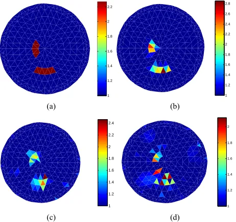
4.2. Two Targets Simulation
The two targets simulation is presented in this section. In the 2-D circular domain, the background resistivity is 1
Ω·m, and the target is 2.3 Ω·m. The setting of the itera-tive initial value and the end condition is same as the setting of the single target simulation.
Figure 5 shows the simulation targets and the recon-struction results under different noise levels. The fitness value and the total error are presented in Table 2. The results show that the reconstruction targets border be-come vague the fitness value and the total error increase gradually with the increase of noise.
5. Conclusions
[image:4.595.59.287.370.592.2]1 1.2 1.4 1.6 1.8 2 2.2
1 1.2 1.4 1.6 1.8 2 2.2 2.4 2.6 2.8
(a) (b)
1 1.2 1.4 1.6 1.8 2 2.2 2.4
1 1.2 1.4 1.6 1.8 2
[image:5.595.59.290.85.303.2](c) (d)
Figure 5. Simulation experiment model and the reconstruc- tion result of the two targets. (a) Simulation target; (b) Re- construction result (non-noise); (c) Reconstruction result (SNR = 40 dB); (d) Reconstruction result (SNR = 30 dB).
Table 2. Fitness value and the total error of the two targets.
SNR (algorithm) Iterations Fitness value Total Error
50 (MPSO) 0.001624 0.001715 Noiseless
60 (MNR) 0.001122 0.000253
50 (MPSO) 0.002360 0.002521 40 dB
60 (MNR) 0.001801 0.000671
50 (MPSO) 0.028320 0.004228 30 dB
60 (MNR) 0.021935 0.003139
avoids the demand of the initial value close to the true value and uses the advantages of the fast convergence speed of MNR algorithm.
The numerical results show that the MPSO-MNR al- gorithm can reflect the resistivity distribution in the so- lution space within the certain iterations. With the target moving to the centre of 2-D solution domain and the in- creasing of the noise, the border of the reconstruction objects becomes vague, and the fitness value and the total error increase gradually. This suggests that the noise and the relative position of target influence the image quality.
Model degeneracy is a general difficulty in optimiz- ing problems. In this paper, the resistivity distribution of the certain configuration can be reconstructed by MPSO- MNR algorithm and the results show changes in per- formance under different noise levels. Therefore, the anti-noise algorithm will be the research direction in the practical application of the EIT. In addition, the effect of ther configurations on MPSO-MNR will be the research
works in EIT as well.
6. Acknowledgements
The authors would like to thank the reviewers whose thoughtful comments added to the efficacy of this paper. This work was supported by foundation of education department of Shaanxi provincial government (No. 2010JK892) and national college’s student innovative project (No. 201210722024).
REFERENCES
[1] H. Dehghani and M. Soleimani, “Numerical Modeling Errors in Electrical Impedance Tomography,” Physiologi- cal Measurement, Vol. 28, No. 7, 2007, pp. S45-S55.
http://dx.doi.org/10.1088/0967-3334/28/7/S04
[2] G.-Z. Xu, Y. Li, et al, “Electrical Impedance Tomography
in Biomedical Engineering,” China Machine Press, Bei- jing, 2010.
[3] W. He, C.-Y. Luo, Z. Xu, et al., “Principle of the Electri-
cal Impedance Tomography,” Science Press, Beijing, 2009. [4] Y. Li, G. Z. Xu, L. Y. Rao, et al., “MNR Method with
Self-Determined Regularization Parameters for Solving Inverse Resistivity Problem,” Proceedings of 27th Annual International Conference of the IEEE Engineering in Medicine and Biology, Vol. 3, 2005, pp. 2653-2655. [5] H. Zhang, Y.-J. Zhou and X.-D. Zhang, “Algorithm Study
of 2-D Electrical Impedance Tomography,” Journal of Xianyang Normal University, Vol. 27, No. 2, 2012, pp. 17-
19.
[6] H. Zhang, X.-D. Zhang, et al., “Electromagnetic Imaging
of the 2-D Media Based on Particle Swarm Algorithm,” 2010 Sixth International Conference on Natural Compu-tation (ICNC), 10-12 August 2010, pp. 262-264. [7] H. Zhang, H. B. Wang, Y. J. Zhou and X. D. Zhang,
“Re-search of Electrical Impedance Tomography Based on the Modified Particle Swarm Optimization,” 2012 Eighth In-ternational Conference on Natural Computation (ICNC),
29-31 May 2012, pp. 1127-1129.
[8] R. Olmi, M. Bini and S. Priori, “A Genetic Algorithm Approach to Image Reconstruction in Electrical Imped-ance Tomography,” IEEE Transactions on Evolutionary Computation, Vol. 4, No. 1, 2000, pp. 83-88.
http://dx.doi.org/10.1109/4235.843497
[9] H. Zhang, Y. Li, X. M. Wang and X. D. Zhang, “MPSO- MNR Algorithm Study of 2-D Electrical Impedance To- mography,” Computer Engineering and Applications,Vol.
49, No. 3, 2013, pp. 29-32.
[10] M. Donelli and A. Massa, “Computational Approach Based on a Particle Swarm Optimizer for Microwave Imaging of Two-Dimensional Dielectric Scatterers,” IEEE Transac- tions on Microwave Theory and Techniques, Vol. 53, No.
5, 2005, pp. 1761-1776.
http://dx.doi.org/10.1109/TMTT.2005.847068
[11] S. Huang, “Regularization Algorithm Research of Static Electrical Impedance Tomography,” Ph.D. Dissertation, Chongqing University,Chongqing, 2005.
[image:5.595.57.286.378.497.2]