The Active for Life Year 5 (AFLY5) school based cluster randomised controlled trial protocol: detailed statistical analysis plan

(1)

U P D A T E

Open Access

The Active for Life Year 5 (AFLY5) school-based

cluster randomised controlled trial protocol:

detailed statistical analysis plan

Debbie A Lawlor

1*

, Tim J Peters

2

, Laura D Howe

1

, Sian M Noble

1

, Ruth R Kipping

1

and Russell Jago

3

Abstract

Background:The Active For Life Year 5 (AFLY5) randomised controlled trial protocol was published in this journal in 2011. It provided a summary analysis plan. This publication is an update of that protocol and provides a detailed analysis plan.

Update:This update provides a detailed analysis plan of the effectiveness and cost-effectiveness of the AFLY5 intervention. The plan includes details of how variables will be quality control checked and the criteria used to define derived variables. Details of four key analyses are provided: (a) effectiveness analysis 1 (the effect of the AFLY5 intervention on primary and secondary outcomes at the end of the school year in which the intervention is delivered); (b) mediation analyses (secondary analyses examining the extent to which any effects of the intervention are mediated via self-efficacy, parental support and knowledge, through which the intervention is theoretically believed to act); (c) effectiveness analysis 2 (the effect of the AFLY5 intervention on primary and secondary outcomes 12 months after the end of the intervention) and (d) cost effectiveness analysis (the cost-effectiveness of the AFLY5 intervention). The details include how the intention to treat and per-protocol analyses were defined and planned sensitivity analyses for dealing with missing data. A set of dummy tables are provided in Additional file 1.

Discussion:This detailed analysis plan was written prior to any analyst having access to any data and was

approved by the AFLY5 Trial Steering Committee. Its publication will ensure that analyses are in accordance with an a priori plan related to the trial objectives and not driven by knowledge of the data.

Trial registration:ISRCTN50133740

Background

The aims and details of data collection for Active For Life Year 5 (AFLY5) are provided in the main trial proto-col paper, which was published in 2011 [1]. This detailed analysis plan is an update to that published protocol. It was written between November-December 2012, with this final version completed in January 2013. This final version of the analysis plan was approved by the AFLY5 Trial Steering committee on 31 January 2013, prior to any of the researchers who will analyse the data having access to any of them.

Whilst the AFLY5 RCT began in May 2011, no data had been seen by any of the authors of this analysis plan at the time of writing. This final version has been submitted to

the Trial Steering Committee Chair–Prof. J. Cade–who will note any subsequent changes to it.

Data, for initial analyses will be released to analysts D. A. Lawlor and L. Howe in the second week in February 2013; they will begin quality control checks and main analysis 1 (see below) then, with input from T.J. Peters and R. Kipping in interpreting results.

Update

The purpose of this update is to provide a detailed analysis plan of the effectiveness and cost-effectiveness of the AFLY5 intervention. This includes details of how variables will be quality control checked and the criteria used to define derived variables. Details of four key analyses are also provided: (a) effectiveness analysis 1 (the effect of the AFLY5 intervention on primary and secondary outcomes at the end of the school year in which the intervention is * Correspondence:[email protected]

1_{School of Social and Community Medicine, University of Bristol, Bristol, UK} Full list of author information is available at the end of the article

(2)

delivered); (b) mediation analyses (secondary analyses exa-mining the extent to which any effects of the intervention are mediated via self-efficacy, parental support and know-ledge, through which the intervention is theoretically be-lieved to act); (c) effectiveness analysis 2 (the effect of the AFLY5 intervention on primary and secondary outcomes 12 months after the end of the intervention) and (d) cost effectiveness analysis (the cost-effectiveness of the AFLY5 intervention). The details include how the intention to treat and per-protocol analyses were defined and planned sensitivity analyses for dealing with missing data. A set of dummy tables are provided in Additional file 1. We begin by tabulating the outcome and mediators and then go onto the detailed analysis plan.

By writing and publishing this analysis plan prior to any analysts having access to AFLY5 data we hope to en-sure that analyses are driven by a priori defined methods related to the trial objectives and not influenced by knowledge of the data.

Outcome and mediation measurements

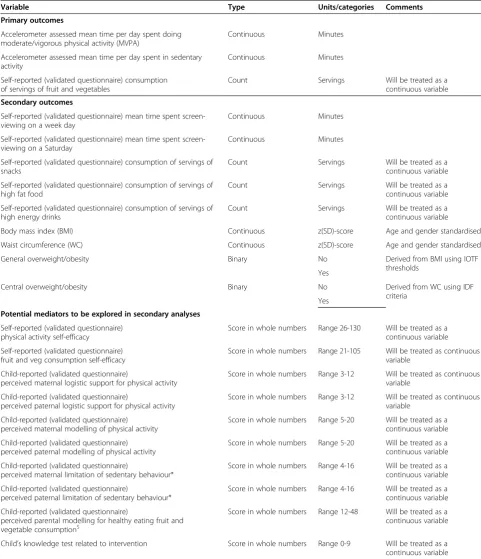
Table 1 lists the primary and secondary outcomes and the hypothesised mediators, and describes the type of variable for each of these.

Detailed analysis plan

The detailed analysis plan is described in the following sections:

1. Quality control checking (QC) and cleaning of data and derivation of new variables from collected (raw) data.

2. Effectiveness analysis 1: The effect of the AFLY5 intervention on primary and secondary outcomes at the end of the school year in which the intervention is delivered.

3. Mediation analyses: Secondary analyses examining the extent to which any effects of the intervention are mediated via self-efficacy, parental support and knowledge, through which the intervention is theoretically believed to act.

4. Effectiveness analysis 2: The effect of the AFLY5 intervention on primary and secondary outcomes 12 months after the end of the intervention. 5. Cost effectiveness analysis: The cost-effectiveness of

the AFLY5 intervention.

Quality checking, cleaning data and deriving variables

Identical cleaning/QC and variable derivation procedures will be used for data that were collected at baseline (com-pleted May–October 2011), first follow-up (com(com-pleted May–September 2012) and second follow-up (planned for February-July 2013).

Accelerometer data

Accelerometer data will be analysed using appropriate software (e.g. Kinesoft).

In both studies of children and adults different methods are used for deriving accelerometer outcome variables in different studies [2-7]. Differences occur in:

The epoch (time) length of recorded bouts of data

What period of records of consecutive zero

movement/counts are taken to indicate a participant has removed the accelerometer (these periods are removed from the calculation of hours wear per day)

Number of hours per day that are considered to

provide valid wake-time wear for derivation of outcomes

Number of days that the accelerometer should be

worn to provide valid total wear time for derivation of outcomes

The thresholds of counts per minute of activity that

are used to define MVPA and sedentary behaviour

Whilst the considerable research in this area highlights how different decisions for these issues result in different mean levels of outcomes [2-7], we could find no evidence that considered what effect (if any) these differences might have on the results in epidemiological association studies or in intervention studies, such as AFLY5. In a well-conducted randomised controlled trial, we would expect all participant characteristics, other than the intervention, to be the same by randomised group (other than differ-ences that may occur due to chance). Thus, the particular accelerometer criteria that are used for all participants in a RCT should not influence the effect of the intervention on outcomes. That is we would expect differences in charac-teristics such as return of accelerometer, wear-time, num-ber of periods of a given time of consistent zero levels of activity, etc., to be similar between children from schools randomised to control and those randomised to the inter-vention. We will test this assumption in AFLY5 (see Sec-tion 2.2 and dummy table in AddiSec-tional file 1: Table S1).

Consequently, in AFLY5 we have selected all criteria related to wear time on the basis of face validity relevant to our study population and consistent with the instruc-tions given to the children about wearing the accelerom-eter, as suggested in a recent review [3].

(3)

[image:3.595.56.538.100.660.2]

Table 1 AFLY5 outcomes and mediators

Variable Type Units/categories Comments

Primary outcomes

Accelerometer assessed mean time per day spent doing moderate/vigorous physical activity (MVPA)

Continuous Minutes

Accelerometer assessed mean time per day spent in sedentary activity

Continuous Minutes

Self-reported (validated questionnaire) consumption of servings of fruit and vegetables

Count Servings Will be treated as a

continuous variable Secondary outcomes

Self-reported (validated questionnaire) mean time spent screen-viewing on a week day

Continuous Minutes

Self-reported (validated questionnaire) mean time spent screen-viewing on a Saturday

Continuous Minutes

Self-reported (validated questionnaire) consumption of servings of snacks

continuous variable

Self-reported (validated questionnaire) consumption of servings of high fat food

continuous variable

Self-reported (validated questionnaire) consumption of servings of high energy drinks

continuous variable

Body mass index (BMI) Continuous z(SD)-score Age and gender standardised

Waist circumference (WC) Continuous z(SD)-score Age and gender standardised

General overweight/obesity Binary No Derived from BMI using IOTF

thresholds Yes

Central overweight/obesity Binary No Derived from WC using IDF

criteria Yes

Potential mediators to be explored in secondary analyses

Self-reported (validated questionnaire) physical activity self-efficacy

Score in whole numbers Range 26-130 Will be treated as a continuous variable

Self-reported (validated questionnaire) fruit and veg consumption self-efficacy

Score in whole numbers Range 21-105 Will be treated as continuous variable

Child-reported (validated questionnaire)

perceived maternal logistic support for physical activity

perceived paternal logistic support for physical activity

Child-reported (validated questionnaire) perceived maternal modelling of physical activity

Child-reported (validated questionnaire) perceived paternal modelling of physical activity

perceived maternal limitation of sedentary behaviour*

perceived paternal limitation of sedentary behaviour*

perceived parental modelling for healthy eating fruit and vegetable consumption$

Child’s knowledge test related to intervention Score in whole numbers Range 0-9 Will be treated as a continuous variable IOTFInternational Obesity Task Force; IDF: International Diabetes Federation.

*For sedentary behaviour we are not aware of any validated questionnaire assessing parental modelling of healthy sedentary behaviour for use in children and so have only collected information regarding maternal and paternal limiting of sedentary behaviour.

$

(4)

to 3,581 counts per minute [6]. External validation studies included more participants than the original calibration studies, but were still of small sample size (n= 30–206), often of poor quality and used a variety of comparison methods [6]. Fewer studies are available of thresholds for defining sedentary behaviour in children. The most recent, and the largest (n= 206) and methodologically most sound external validation study to date [7], suggested that the thresholds recommended by Evenson [8] were most valid. We will therefore use the Evenson thresholds for MVPA (≥2,296 counts per minute) and sedentary behaviour (0–100 counts per minute) in AFLY5.

Further considerations in choosing which criteria to use for deriving accelerometer outcomes are the import-ance of minimising chimport-ance findings due to multiple test-ing and of potentially compromistest-ing statistical efficiency by excluding too many participants for not having valid wear data. We will compare accelerometer characteris-tics by randomised group to test our assumption that these are similar.

Criteria that will be used in AFLY5 for deriving accelerometer outcome measurements

Data collected in 10-s epochs

A period of≥60 min of consecutive 0 counts

assumed to be non-wear and these periods removed from the measurement of wear-time

≥8 h per day to be considered to have valid

wear-time for a given day

≥3 valid days in total

MVPA defined as≥2,296 counts per minute

Sedentary behaviour defined as 0 to 100 counts

per minute

Once the key outcomes–time spent in MVPA and in sedentary behaviour – have been derived using the ac-celerometer software they will be exported from that software into Stata, and ‘general’cleaning and checking of the distributions of these variables will be undertaken.

Cleaning/QC of the accelerometer derived variables will include

Normal plots, histograms and scatter plots will be

used to identify potentially implausible measurements.

Scatter plots will compare for each variable its baseline and follow-up value and also will compare different variables measured at the same time point that would be expected to be moderately to strongly correlated; time spent in MVPA to time spent in sedentary behaviour, time spent in MVPA to weight and time spent in sedentary behaviour to weight.

Values that appear outside of the main distribution in the majority of participants (i.e. outliers) on normal plots and histograms will be assumed to be correct if the scatter plots show consistency–e.g. lying close to the main‘line’of positive association for the same variable measured at baseline and again at follow-up or the inverse association of time in MVPA with time in sedentary behaviour and close to the main‘line’of inverse association of time spent in MVPA with weight.

Outliers that deviate from the‘line’of the scatter plots by 2 SD or more on either axis will be considered implausible.

For implausible values, the original data will be checked in the accelerometer software to make sure criteria have been applied correctly and any errors will be corrected.

For remaining implausible values a variable that

indicates‘possible implausible value ofX’ (whereXis the name of the variable that has a possible implausible value) will be derived.

In the main effectiveness analyses we will complete analyses with all participants (including where they have a possible implausible value) included and again with participants excluded for analyses with a given outcome if their value for that outcome has been marked as possibly implausible.

If removal of participants with possible implausible values results in a change of a magnitude that for that outcome would affect the interpretation/ conclusion for that outcome then both sets of results will be reported; otherwise only the results with all included irrespective of ‘implausible value’ status will be reported.

Diet data

Questionnaire responses are entered into a Microsoft Access database.

Initial cleaning

(5)

remaining words that cannot be deciphered. Words that remain impossible to decipher after all attempts are possible servings of food/drink that cannot be included further in any analyses.

Coding of diet data

After initial cleaning, codes are applied that indicated which (if any) outcome category – fruit and vegetables, snacks, high fat foods and high energy drinks – each food item belongs to. These codes are allocated follow-ing the validated scorfollow-ing system developed by the inves-tigators who developed the questionnaire [9]. Codes are allocated by one individual, with a random 5% coded independently by a second individual. Discrepancies of greater than 5% in this second coding would trigger re-coding of all data and a detailed check of why inconsist-encies have occurred. Full details of how each food item is coded are provided in Additional file 2.

Final cleaning

Final cleaning will include:

Exploring the distribution of the diet score (number

of servings) for each of the four types of food used as an outcome in our study (fruit and vegetables, snacks, high fat foods and high energy drinks) using bar charts.

Checking implausibly high values (for any of these

scores it is possible for a child to eat no portions on a day, whereas very high values are more likely to be implausible).

A priori we consider implausibly high values > 8 portions/day for any single outcome.

Any possible implausible values will be checked by

going back to the original questionnaire responses and coding for that questionnaire, with corrections made as appropriate.

Screen viewing data

Cleaning/QC of the screen viewing data will include:

Scatter plots will compare self-reported time spent screen-viewing at baseline to the same at follow-up and will also compare self-reported time spent screen-viewing at both time points on weekdays to that on Saturdays and also both to time spent in sedentary behaviour based on the accelerometer data.

Values that appear outside of the main distribution in the majority of participants (i.e. outliers) on normal plots and histograms will be assumed to be correct if the scatter plots show consistency.

For implausible values, the original data will be checked on the completed questionnaires and any transcription errors corrected.

If removal of participants with possible implausible values results in a change of a magnitude that for self-reported screen viewing would affect the interpretation/conclusion for that outcome then both sets of results will be reported; otherwise only the results with all included irrespective of

‘implausible value’status will be reported.

Anthropometric data

Cleaning of data

The following will be undertaken for QC and cleaning data:

Scatter plots will compare each measure at baseline

(6)

majority of participants (i.e. outliers) on normal plots and histograms will be assumed to be correct if the scatter plots show consistency.

The original data collection sheets for these values will be checked and if these show that the data have been incorrectly entered in the database this will be corrected.

Derivation of variables

The age range of the participants in this study at any one time point of data collection is narrow, because they are all from the same school year. However, over time children will age by on average 3 years. Because of the marked variability of body mass index (BMI) and waist circumference (WC) with age and gender we will derive internally standardised z-scores (also known as standard deviation scores) at each time point of data collection as follows:

z−scoreBMI¼ðoBMIag–mBMIagÞ sdBMIag

z−scoreWC¼ðoWCag–mWCagÞ sdWCag

Where:

oBMIagis the observed BMI for a participant of a given gender and age (within 6 month age categories)

mBMIagis the mean BMI for participants of the same

gender and same age (within 6 month age categories) as a given participant for whom the score is being derived sdBMIagis the standard deviation of the mean BMI for participants of the same gender and same age (within 6 month age categories) as a given participant for whom the score is being derived

oWCagis the observed WC for a participant of a given gender and age (within 6 month age categories)

mWCagis the mean WC for participants of the same

gender and same age (within 6 month age categories) as a given participant for whom the score is being derived

sdWCagis the standard deviation of the mean WC for

participants of the same gender and same age (within 6 month age categories) as a given participant for whom the score is being derived

The binary anthropometric outcomes will be derived using:

International Obesity Task Force (IOTF)

age- (in 6 months) and gender-specific thresholds for overweight and obesity derived from BMI in children (general overweight/obesity) [10].

For WC any participant above the 90th percentile

for age- and gender-specific values derived from UK relevant centiles [11] will be defined as having central overweight/obesity, as suggested by the International Diabetes Federation (IDF) [12].

Self-efficacy variables

Physical activity self-efficacy is assessed with a 26-item scale with each item having a five-point (1 to 5) score option (higher values indicating greater self-efficacy) [13]. Thus, the possible range of total scores is 26–130.

Fruit and vegetable self-efficacy is assessed with a 21-item scale with each 21-item having a five-point (1 to 5) score option (higher values indicating greater self-efficacy) [14]. Thus, the possible range of total scores is 21–105.

Initial cleaning–dealing with missing data and deriving score

For these self-efficacy scores there are generally two types of missing data: (1) complete missing data (i.e. because the child was not present in school when data were collected; so far no child who was present has refused to complete the questionnaire) and (2) partial missing data where the child has completed some but not all items of the questionnaire. This section describes how we will deal with partial missing data only and hence derive a score for all children who have completed some of the ques-tionnaire. Dealing with complete missing questionnaire data is addressed in the main analyses sections under ‘dealing with missing data’(see below).

For both scores we will initially check for item missing data – i.e. the extent to which a child who has com-pleted some of the questions for a given score has left some of the items blank.

(7)

emphasis placed on completing every item we anticipate that there will be very few missing data.

Where data appear to be missing the original ques-tionnaires will be checked to make sure this is not a data entry error. Any such errors will be corrected.

From the baseline assessment of these self-efficacy mea-surements we know that missing data are rare–85% have complete data for all items, 10% missing just one item, 3% missing two items and 2% missing three or more items.

To deal with item missing data we will do the following:

Any participant missing three or more items will be

identified with a variable (derived variable indicating

‘high level of missing data forX’, whereXis the specific self-efficacy measure affected)

For all participants (irrespective of how many items are missing) a final score that takes account of missing data will be generated as follows:

Self efficacy score¼∑IoþðNmð∑IoNoÞÞ

Where

Io = all observed items

No = number of observed items Nm = number of missing items

i.e. the score is the total sum of all observed scores plus the sum of missing scores with missing scores replaced with the mean of observed scores. So for example for a child who has completed 22 items out of the 26 for physical activity efficacy and has a sum of these 22 completed items of 78 the final score will be 78 + (4 × (78 ÷ 22)) = 81.5

In the secondary analyses when we are exploring the

role of these self-efficacy variables as mediators we will complete analyses with all participants [including where they have a‘high’level of missing (defined as above–missing three or more items) for the self-efficacy variable being considered] included and again with participants excluded for a given analysis if they have a high level of missing for the self-efficacy variable.

If removal of participants with‘high levels of item missing data’for a given self-efficacy variable results in a change of a magnitude that would affect the interpretation/conclusion for that mediator (or for its effect on an outcome) then both sets of results will be reported; otherwise only the results with all included irrespective of ‘high levels of item missing data’status will be reported.

Final cleaning

The following will be undertaken:

Scatter plots will compare self-efficacy variables at baseline and follow-up and will also compare the following within each time point; physical activity and fruit and vegetable self-efficacy (which we would expect to be positively associated), physical activity self-efficacy with accelerometer-assessed time spent in MVPA and fruit and vegetable self-efficacy with total portions of fruit and vegetables consumed.

Values that appear outside of the main distribution in the majority of participants (i.e. outliers) on normal plots and histograms will be assumed to be correct if the scatter plots show consistency.

Outliers that clearly deviate from the‘line’of scatter plots will be considered implausible.

The original data collection sheets for these values will be checked and if these show that the data have been incorrectly entered in the database this will be corrected.

suggests‘possible implausible value’will be derived.

In the main effectiveness analyses we will complete analyses with all participants (including where they have a possible implausible value) included and again with participants excluded for a given analysis if they have an implausible indicator for a particular outcome.

As with the high levels of item missing data analyses we will compare the effect of the intervention on each self-efficacy mediator variable with and without those with‘possible implausible values’removed. If removal changes the size of the effect by an amount that would change the interpretation/conclusion of the results analyses with and without these participants removed will be presented; otherwise only those with the participants included.

Parental support variables

The parental support questionnaire for physical activity/ sedentary behaviour [15,16] has items that provide infor-mation (and scores) for the child’s self reported percep-tion of:

(1)Maternal logistic support/encouragement for physical activity (3 items of 4 options; range of possible scores 3–12)

(2)Paternal logistic support/encouragement for physical activity (3 items of 4 options; range of possible scores 3–12)

(8)

(4)Paternal modelling of physical activity (5 items of 4 options; range of possible scores 5–20)

(5)Maternal restriction of sedentary behaviour (4 items of 4 options; range of possible scores 4–16)

(6)Paternal restriction of sedentary behaviour (4 items of 4 options; range of possible scores 4–16)

The parental support questionnaire for fruit and vege-table consumption has items that provide information for parental modelling of healthy behaviour for both par-ents combined [17]. The questionnaire consists of 12 items each of which has 4 options and hence this score has a range of possible values from 4 to 48. We were unable to identify a validated questionnaire for parental logistic support of fruit and vegetable consumption that was suitable for children to complete and the question-naire that we have for parental modelling is with both parents combined.

Initial cleaning–dealing with missing data and deriving score

For these parental support scores there are generally two types of missing data as described above for the self-efficacy scores (note whilst these questions relate to paren-tal support all questions were completed by the children in the classroom with no input from parents).

For all seven scores (6 related to physical activity and 1 to fruit and vegetable consumption) we will initially check for missing data –i.e. the extent to which a child has not completed all of the items for each score.

Since the questionnaire is completed by the children with the fieldworkers present in the classroom and em-phasis placed on completing every item, we anticipate that there will be minimal missing data. For the physical activity variables that are collected separately for both parents we anticipate missing data will be greater for fa-thers than mofa-thers, as some children may have limited contact with their fathers. The baseline data collection confirms this, with complete data on physical activity/ sedentary behaviour support scores for mothers being provided by 90-92% of participants and for fathers for 82-84% of participants.

Because there are only a small number of items for each of the physical activity/sedentary behaviour parental sup-port scores and hence the range of options is small, to deal with the small number of participants we anticipate will have some partial missing data we will:

Generate a mean score for each child irrespective of

the number of items completed (e.g. if a child has completed all 3 of the logistic modelling items their score will be the sum of each score divided by 3; if they have completed only 2 their score will be the sum of the 2 divided by 2)

Generate a variable that indicates some missing data

for any of the scores (i.e. whether the child has 1 or more items missing for any of the physical activity/ sedentary parental support scores they will be indicated as having some missing).

In the main mediator analyses all participants will be included for any given physical activity/sedentary behaviour parental support score irrespective of whether they had some missing data or not. The analyses will then be repeated with those who had some missing data excluded from analyses with that particular score.

If removal of participants with‘high levels of item missing data’for a given parental support variable results in a change of a magnitude that would affect the interpretation/conclusion for that mediator (or for its effect on an outcome) then both sets of results will be reported; otherwise only the results with all included irrespective of ‘high levels of item missing data’status will be reported.

For the parental modelling of fruit and vegetable

consumption the number of items and range of potential scores is relatively large and we will approach item missing data in this variable in the same way as that for the self-efficacy variables described above, i.e.:

Any participant missing three or more items for the

parental modelling of fruit and vegetable score will be identified with a variable (derived variable indicating‘high’level of missing data).

For all participants (irrespective of how many items are missing) a final score that takes account of missing data will be generated as follows:

Parental support score¼∑Io

þðNmð∑IoNoÞÞ

Where

Io = all observed items

No = number of observed items Nm = number of missing items

i.e. the score is the total sum of all observed scores plus the sum of the mean of observed scores for any with a missing score. So a child who has completed 11 items out of the 13 items for parental modelling of health fruit and vegetable consumption where the sum of these 13 completed items is 28 will have a final score of 28 + (2 × (28 ÷ 13)) = 30.2

In the main mediator analyses we will complete

(9)

If removal of participants with‘high levels of item missing data’for the parental modelling of fruit and vegetables variable results in a change of a magnitude that would affect the interpretation/conclusion for this mediator (or for its effect on an outcome) then both sets of results will be reported; otherwise only the results with all included irrespective of‘high levels of item missing data’status will be reported.

Final cleaning of all parental support scores The following will be undertaken:

Means, median, SD, IQR and full range,together

with normal plots and histograms will be examined. As with the physical activity/sedentary behaviour scores any values outside the possible range must be an error in summing/generating the final score and will therefore be checked by looking at the Stata code used for doing this.

To check for implausible values within the range

expected relationships between variables will be checked by looking at scatter plots between each of the variables when measured at baseline and at follow-up and also between variables at the same time point as follows: physical activity/sedentary behaviour parental support and the fruit and vegetable support scores, using scatter plots. Where these suggest unlikely values for any participant (deviation from the scatter predicted line of association of more than 2 SD on either axes) the data entered values for each item will be compared against the original questionnaires and any entry errors corrected.

For remaining unlikely values after these checks a variable that indicates‘possible implausible value’ will be derived.

In the main effectiveness analyses we will complete analyses with all participants (including where they have a possible implausible value) included and again with participants excluded for a given analysis if they have an implausible indicator for a particular outcome.

As with the high levels of item missing data analyses we will compare the effect of the intervention on each mediator variable with and without those with

‘possible implausible values’removed. If removal changes the size of the effect by an amount that would importantly influence the interpretation or conclusion of results both sets of results will be presented; otherwise only the ones with no exclusion.

Child’s knowledge

At the two follow-up assessments we will collect data on the child’s knowledge in relation to what they have been

taught in the intervention schools as part of the inter-vention. This measurement was not originally planned but as a study team we felt it was important to test whether specific knowledge is greater in children from the intervention schools than in those from the control schools after the intervention. We developed a question-naire that reflects knowledge that the intervention les-sons and homework aim to provide the children with (Additional file 3). This was developed by the study team with feedback from year 5 teachers and piloting (to test whether the questions were understood) amongst chil-dren aged 8–10 who were known to members of the study team. The questionnaire consists of nine multiple-choice questions. Children are instructed to tick one answer only from the three choices provided for each question. The range of scores possible is therefore from 0 to 9. We will deal with possible item-missing data for this knowledge test in exactly the same way as that de-scribed above for the parental support of physical activ-ity/sedentary activity. QC checks will also be similar to those described above, although here we have no base-line measure with which to check likely outliers.

Effectiveness and mediation analyses

The next sections describe the methods that will be used to analyse the effect of the intervention and whether this effect is mediated by measurements that indicate the pathways through which the intervention should, in the-ory, operate.

Three separate analyses will be undertaken and most likely presented in separate research publications:

1. Effectiveness analyses 1, which determines the effect of the‘immediate’effect of the intervention–i.e. the effect on outcomes assessed at the end of the school year during which the intervention has been delivered.

2. Mediation analyses. These are secondary analyses as they were not planned at the time of submission of the grant application and were not taken into account in the trial sample size calculation. The justification for undertaking these analyses is provided below. They will examine the extent to which any immediate effect of the intervention is mediated by measurements of the pathways through which the AFLY5 intervention is theorised to work. 3. Effectiveness analyses 2, which determined the‘

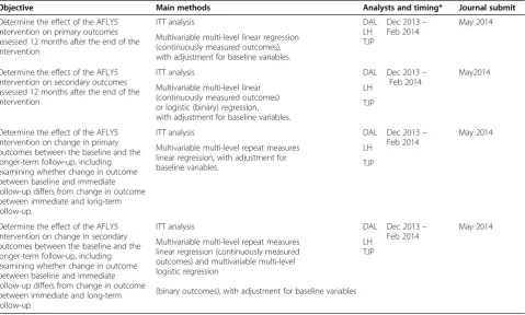
long-term’effect of the intervention–i.e. the effect on outcomes assessed 12 months after the end of the school year in which the intervention was delivered.

(10)

specific aspects of the analyses that are unique to ana-lyses 2 and 3 above. Dummy (empty) tables for these analyses are provided as examples in Additional file 1.

Although we initially planned that these analyses would be done with the analysts blind to which schools were intervention and which were control, this will not be done (analysts will know which schools are which). This is because the per-protocol analyses can only be done by knowing the number of lessons taught in each interven-tion school and therefore removes any possible ‘blinding’ of the analyst.

Effectiveness analyses 1: the immediate effect of the AFLY5 intervention on primary and secondary outcomes (i.e. effect at the end of the school year of the intervention)

The main effectiveness analysis paper will be written according to the“Consort 2010: extension to cluster ran-domised trials”statement [18].

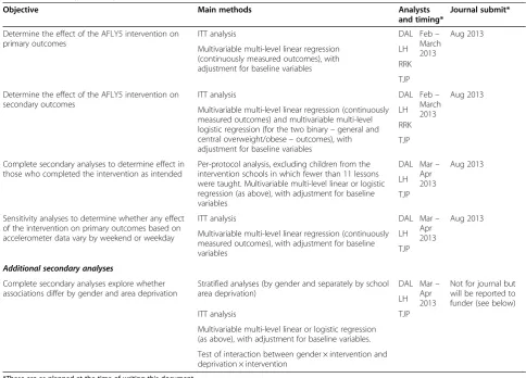
Table 2 summarises the objectives, methods and plan-ned timelines for this analysis.

This analysis is primarily concerned with the ‘imme-diate’ effectiveness of the intervention, with outcomes

assessed ~12 months after the baseline assessment/ran-domisation (which corresponds to the immediate end of the intervention period).

Comparison of baseline characteristics and extent of missing follow-up data between intervention and control groups We will compare relevant summary statistics of baseline characteristics between participants in schools who were allocated to be an intervention school and those allocated to be a control group in order to determine whether any potentially influential imbalance has occurred (by chance) between these two groups. These comparisons will also include accelerometer characteristics, including wear-time, time with consecutive zero levels of activity, etc., to test our assumption that the characteristics that are used in cri-teria for deriving the accelerometer variables do not vary by randomised group (see Section 1 above).

[image:10.595.54.539.365.713.2]

For all continuous and score variables we will check dis-tributions using histograms and normal plots to examine how close to normality these are before deciding which summary statistics to present (see bullet points below).

Table 2 Summary of analysis 1–effectiveness at 12 months

Objective Main methods Analysts

and timing*

Journal submit*

Determine the effect of the AFLY5 intervention on primary outcomes

ITT analysis DAL Feb_–

March 2013

Aug 2013

Multivariable multi-level linear regression (continuously measured outcomes), with adjustment for baseline variables

LH

RRK

TJP

Determine the effect of the AFLY5 intervention on secondary outcomes

ITT analysis DAL Feb_–

March 2013

Aug 2013

Multivariable multi-level linear regression (continuously measured outcomes) and multivariable multi-level logistic regression (for the two binary–general and central overweight/obese–outcomes), with adjustment for baseline variables

LH

RRK

TJP

Complete secondary analyses to determine effect in those who completed the intervention as intended

Per-protocol analysis, excluding children from the intervention schools in which fewer than 11 lessons were taught. Multivariable multi-level linear or logistic regression (as above), with adjustment for baseline variables

DAL Mar_– Apr 2013

Aug 2013

LH

TJP

Sensitivity analyses to determine whether any effect of the intervention on primary outcomes based on accelerometer data vary by weekend or weekday

ITT analysis DAL Mar–

Apr 2013

Aug 2013

Multivariable multi-level linear regression (continuously measured outcomes), with adjustment for baseline variables

LH

TJP

Additional secondary analyses

Complete secondary analyses explore whether associations differ by gender and area deprivation

Stratified analyses (by gender and separately by school area deprivation)

DAL Mar_– Apr 2013

Not for journal but will be reported to funder (see below) LH

ITT analysis TJP

Multivariable multi-level linear or logistic regression (as above), with adjustment for baseline variables.

Test of interaction between gender × intervention and deprivation × intervention

*These are as planned at the time of writing this document.

(11)

The comparisons between the two groups will be made by summarising variables in each group (randomised versus control schools):

Continuous variables that we anticipate will have approximately normal distributions (likely to include age, accelerometer time spent in MVPA, time spent in sedentary behaviour, BMI z-scores, WC z-scores) will be presented as means and standard deviations (SD).

Continuous variables/scores that we anticipate will not have an approximate normal distribution (likely to include self-reported time spent screen viewing, self-efficacy scores for both physical activity and fruit and vegetables, parental modelling scores for fruit and vegetables) will be presented as medians and interquartile ranges (IQR).

Binary/categorical variables (general overweight/

obesity, central overweight/obesity, school

involvement in other health promoting activities and school area deprivation) will be presented as number (N) and percentage (%).

We will not compare baseline characteristics between the two groups with a statistical test (p-value) as any low values simply represent a type-1 error under the as-sumption that we have adequately randomly allocated participants [19]. As described in the general study protocol paper our procedures for randomly allocating schools to control or intervention were adequate [1].

Additional file 1: Table S1 illustrates how the compari-son of baseline characteristics will be presented.

Dealing with missing data

Missing baseline data Any child from a randomised

school with any baseline measure is a recruited study participant.

Numbers with valid data for each of the baseline mea-surements are likely to vary. For example, numbers with accelerometer data are likely to be lower than for other measurements because some participants will not have worn their accelerometer for sufficient time for data to be valid and some may not return their accelerometer. Numbers with BMI and WC measurements may be lower than for the dietary outcomes because some chil-dren may not provide assent for these measures. We an-ticipate that proportions with missing data for any particular measure will be similar in the two randomised groups but will check this (see Figure 1).

Intention-to-treat analyses and dealing with missing follow-up outcome data

For the main analyses we will use intention to treat (ITT). ITT requires all participants in a clinical trial to

be included in the main analyses in the groups to which they were randomised [20,21]. This is straightforward if there is no loss to follow-up or missing data on some outcomes at follow-up amongst those who have been randomised, but is less straightforward where there is loss to follow-up/missing data [20,21]. A four-point framework for dealing with missing outcome data has recently been proposed to deal with this issue [20,21]. It emphasises the fact that all approaches (including complete case analysis–i.e. only including those with observed outcome data) – rely on assumptions that in any given situation may be more or less plausible but are always untestable. It therefore cautions against a‘one size fits all’, but suggests using the most plausible assumptions about the nature of missing data and then testing these assumptions in sensi-tivity analyses; in particular it notes that in many cases the most plausible assumptions would support analyses on those with observed data using either mixed (multilevel models) or complete case analyses [20,21].

Complete case analyses and several of the common methods for imputing/dealing with missing data, includ-ing the multilevel linear regression model that we will use here for all primary outcomes, assume that missing

Eligible schools for randomisation N = 60

Intervention Schools N = 30 Baseline Measure Np

Total

Accelerometer

Diet

Weight & Height

Waist

Screen time

Control Schools N = 30 Baseline Measure Np

Total

Accelerometer

Diet

Weight & Height

Waist

Screen time

Randomisation

Intervention Schools N = 30 Follow-up measure Np (%)

Total

Accelerometer

Diet

Weight & Height

Waist

Screen time

Control Schools N = 30 Np (%)

Total

Accelerometer

Diet

Weight & Height

Waist

Screen time

[image:11.595.305.538.87.357.2]

Follow-up measure

(12)

data are missing at random (MAR). That is, missing values in participants with missing data are assumed to be similar to observed values in participants with similar levels of other variables that are observed in other par-ticipants (i.e. missing is independent of unobserved char-acteristics). Another way of thinking about this is that the effect of a randomised intervention is the same in those with missing data as in those without missing data. Having similar proportions of participants with missing data in each arm of a trial is reassuring with respect to the MAR assumption being correct, but is not a guaran-tee, as the plausible reasons for missing data in each arm could be different but result in similar proportions with missing.

In AFLY5, we minimise the extent of missing data through catch-up data collection–i.e. for each participat-ing school at each phase of data collection there is a day for main data collection, but some children may be absent from school on that day; therefore for each school we have ‘catch-up’ days to obtain data on these children. As a result the likely reasons for missing follow-up data for ALL outcomes (i.e. where a child is not seen at all at one of the follow-up phases) are that the child moves school between data collection phases or the child is absent from school for a prolonged period or frequently so that they miss the main and catch-up data collection days. Missing one or more (but not all) of the specific measurements at follow-up could occur if the child does not give assent, or for the accelerometer-based outcomes the child does not return the accelerometer or does not wear it for a required period of time. In the case of the AFLY5 RCT, MAR is plausible since random-isation is at the level of the schools, parental opt-out consent is ascertained at the start of the study and relevant for all data collection times, and it is implausible that the delivery of the intervention lessons and homework in the intervention schools or lack of these in the control groups would affect the likelihood of a child being absent on days of data collection, declining assent for a particular meas-ure or not returning the accelerometer or wearing to for the required time. Information from the local councils suggests that movement between schools is relatively low, but it is possible that children who move may differ from those who do not on the basis of unobserved characteris-tics. Children who move school might be from families who are relatively unorganised with children often moving school or they could be from families who move their child from state to private school in year 6 in order to attend private secondary school (Bristol has a higher than average for the UK proportion of children in pri-vate secondary school education). The possibility that these types of missing data might bias our findings if not explored will be assessed in sensitivity analyses (see sensitivity analyses 3 and 4 in Table 3).

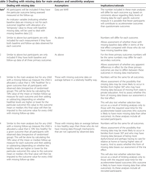
Table 3 details how missing baseline and follow-up out-come data will be managed in the main analyses and a series of sensitivity analyses that aim to test the assump-tions regarding missing data.

In the main analyses we will use multilevel linear re-gression models accounting for the clustered nature of the data in AFLY5. For the main approach to all analyses any child with the measured outcome at follow-up will be included; we will do these analyses for each outcome separately so numbers included in the analyses between each outcome may vary. In order to include all children with the follow-up outcome measure (including those with a missing baseline value) and also be able to take account of the baseline value, we will use the method suggesting by White and Thompson for dealing with missing baseline values [22] in the first (immediate) ef-fectiveness analyses and the mediation analyses. In the second (long-term) effectiveness analyses, we will use a repeated measures multilevel modelling approach to examine differences between randomised groups in the change in outcomes over time from baseline, and so missing data at baseline will be taken into account within these models. Both of these approaches assume data are MAR and in addition to these main analyses a number of sensitivity analyses will be undertaken; see Table 3.

Effect analyses

For the continuously measured outcomes (all primary outcomes and most of the secondary outcomes) we will:

Use normal plots and histograms to assess normality

of the follow-up measure of the outcome. If variables are approximately normally distributed they will be used as they are (i.e. with no

transformation). If they are clearly non-normal we will explore transforming them to improve

normality of the residuals in the regression models. The choice of whether or not to transform variables, and if so which transformation to use, will be decided by considering: (1) the distribution of the variable, (2) the distribution of residuals from regression models, (3) the ease of interpreting results following any given transformation compared with no transformation and (4) whether main results/conclusions are influenced by the

(13)

transformation and compare results with and without this transformation. If the overall

conclusion is not altered by whether the variable is

transformed or not, we would use the

[image:13.595.61.535.89.647.2]

untransformed (easier to interpret) version. Where variables have been log-transformed, the resulting Table 3 Dealing with missing data for main analyses and sensitivity analyses

Dealing with missing data Assumptions Implications/rationale

Maina All participants will be included if they have the particular outcome being assessed measured at the follow-up.

Data are MAR The number included in these main analyses will differ for each outcome e.g. based on comments above regarding likely levels of missing data for each specific outcome measure it is possible that fewer participants will contribute to accelerometer outcomes than questionnaire outcomes

An indicator variable (indicating whether baseline data are missing or not for each outcome) together with allocation of a

‘temporary’value to those with baseline missing data, will be used to deal with missing baseline data [22]

S1 Similar to above but participants are only included for each measurement if they have both baseline and follow-up data observed for each outcome

As above Numbers will differ for each outcome.

Allows assessment of whether those with missing baseline data differ in terms of the trial effect compared with those who do not have missing baseline data

S2 Similar to above but participants are only included if they have both baseline and follow-up data of all three primary outcomes

As above For the three primary outcomes numbers will be the same numbers may differ for each secondary outcome.

Allows assessment of whether any apparent differences in effect for the three primary outcomes are due to differs between these outcomes in missing data mechanisms

S3 Similar to the main analyses but for any child with a missing follow-up measure the child is allocated a value that is 10%‘healthier’for a given outcome than all participants with observed data (irrespective of randomised group). This will be done by calculating the 10% value of the mean or median follow-up measure for each outcome and then adding or subtracting (depending on whether healthier levels are higher or lower for the particular outcome) this value to the outcome mean or median; this final value will then be imputed to the outcome value for every child with missing follow-up data.

Those with missing outcome data on average behave in a relatively healthy way.

Numbers will be the same for all outcomes.

Allows assessment of the possibility that missing data may be more likely to occur in families from higher SEP who may have missing data because of moving from state to private education. And to assess whether this form of missing data biases our assessment of the trial effect.

This will also test whether selection bias occurs as a result of limiting analyses only to those with the required wear-time for the accelerometer based outcomes (this outcome is likely to have more missing data than other outcomes). As these analyses include all recruited participants.

S4 Similar to the main analyses but for any child with a missing follow-up measure the child is allocated a value that is 10%‘less healthy’for a given outcome than all participants with observed data (irrespective of randomised group). This will be done by calculating the 10% value of the mean or median follow-up measure for each outcome and then adding or subtracting (depending on whether less healthy levels are higher or lower for the particular outcome) this value to the outcome mean or median; this final value will then be imputed to the outcome value for every child with missing follow-up data

Those with missing data on average behave in less healthy ways than those who do not have missing data through mechanisms that are not captured by observed data

Numbers will be the same for all outcomes.

Allows assessment of the possibility that missing data may be more likely to occur in families from lower SEP and who may have missing data because of being more dysfunctional and perhaps having to care for a relative at home or having higher rates of truancy. And to assess whether this form of missing data biases our assessment of the trial effect.

This will also test whether selection bias occurs as a result of limiting analyses only to those with the required wear-time for the accelerometer-based outcomes (this outcome is likely to have more missing data than other outcomes). As these analyses include all recruited participants

a

Note for other baseline characteristics that will be included in the model (gender, age and the school stratifying variables–school involvement in other health promoting activities and area deprivation) there should be no missing data. Thus, using a method that allows inclusion of those with missing baseline data in this analysis allows all recruited participants who have an outcome measure to be included in the analyses.

(14)

coefficients will be converted to differences in means on a % scale.

Use multilevel multivariable linear regression to determine the difference in means between participants from schools allocated to the intervention and those allocated to control (reference group = control schools) whilst taking account of clustering (non-independence) amongst children from the same school.

The analyses will include adjustment for the following baseline and stratifying covariables: age, gender, the baseline measure of the outcome being analysed (i.e. for the effect of the intervention on time spent in MVPA we will include baseline MVPA in the model and so on), school involvement in other health promoting activities and school area deprivation.

The model for the main effect of the intervention

on the continuously measured outcomes is

Yijp¼β₀þβ₁X1ijpþβ₂X2ijpþβ₃X3ijpþβ₄X4ijp

þβ5X5ijpþβ6X6ijpþβ7X7ijpþβ8X7ijp

X4ijpþCijþЄijp

Where

Yijpis the outcome for participant

p= 1………m, in thejth schoolj= 1

………..60 in intervention groupi= 1, 2 β0is the intercept, i.e. the outcome amongst those

in intervention schools with the lowest level of all continuously measured covariables, the reference category for all categorical covariables and in school coded 1

β1is the treatment effect (i.e. the mean difference

in outcome comparing pupils from intervention schools to those form control schools) having adjusted for baseline characteristics and taken account of non-independence amongst children from the same school

Χ1ijp¼ 1 if i¼1ðintervention schoolÞ

2 if i¼0ðcontrol schoolÞ

β2toβ6are the adjusted associations of the

baseline and stratifying covariables X2ijpto X6ijp

with the outcome [i.e. age, gender, baseline measure of the outcome (X4ijp), school

involvement in other health promoting activities and school area deprivation]

β7is the association of the indicator variable X7ijp,

indicating missing baseline measure of the outcome, with the follow-up outcome.

β8is the interaction coefficient for the interaction

of the missing baseline indicator variable with the baseline measure of the outcome (X7ijp*X4ijp)

Cijis the school level effect for the schooljth school in intervention groupi

and Cij~ N(0,σ2A)

Єijpis the residual of the outcome for participant

pfrom thejth school in intervention groupi andЄijp~ N(0,σ2W)

and CijandЄijpare independent of each other.

For the binary outcomes (two secondary outcomes – general and central overweight/obesity):

The approach will be broadly similar to that above

described for continuously measured outcomes.

A multilevel multivariable logistic regression model will be used to calculate the odds ratio of binary outcomes children in intervention schools to those in control schools (reference category), whilst taking account of clustering within schools.

Baseline covariables identical to those listed above will be included.

Thus, the model for binary outcomes is

πijp¼Pr Yijp¼1¼logit−1 β₀þβ₁X1ijp

þβ2X2ijpþβ3X3ijpþβ4X4ijpþβ5X5ijp

þβ6X6ijpþβ7X7ijpþβ8X7ijpX4ijpþCij

þЄijp

Where

πijpis the probability that participant

p= 1………m, in thejth schoolj= 1

………..60 in intervention groupi= 1, 2 is overweight or obese

β0is the intercept, i.e. the probability of normal

weight amongst those in intervention schools with the lowest level of all continuously measured covariables, the reference category for all categorical covariables and in school coded 1 β1is the treatment effect (i.e. the log odds of each

binary outcome comparing pupils from intervention schools to those form control schools) having adjusted for baseline and stratifying covariables (as above) and taken account of non-independence amongst children from the same school

Χ1ijp¼ 1 if i¼1ðintervention schoolÞ

2 if i¼0ðcontrol schoolÞ

β2toβ6are the adjusted associations of the

(15)

other health promoting activities and school area deprivation)

β7is the association of the indicator variable

X7ijp, indicating missing baseline measure of the

outcome, with the follow-up outcome. β8is the interaction coefficient for the

interaction of the missing baseline indicator variable with the baseline measure of the outcome (X7ijp*X4ijp)

Cijis the school level effect for the schooljth school in intervention groupi

Єijpis the residual of the outcome for participant

pfrom thejth school in intervention groupi

For all nine secondary outcomes statistical significance will be indicated by a two-sided p-value of≤0.01 (the equivalent of 0.05 following Bonferroni correction for multiple testing; the actual value of the Bonferroni cor-rection 0.05/9 = 0.006, but we have rounded this up to 0.01) [1]. In order to aid interpretation we will present results by multiplying the p-value by 9 in journal publi-cations for these secondary outcomes.

The trial sample size calculations for all outcomes took account of intraclass correlation coefficients calculated using our pilot/feasibility study data [1].

Empty example tables for the main and four sensitivity analyses of the effect of the intervention on primary and secondary outcomes are shown in Additional file 1: Tables S2 to S6.

Secondary per-protocol analyses to determine effect in those who completed the intervention as intended

A per-protocol analysis of the effect completing at least 70% of the lessons will be undertaken by:

Including all children from control schools and only

those children from intervention schools in which at least 70% of the lessons had been taught (i.e. at least 11 of the 16 lessons were taught).

Children from schools that were randomised to the

intervention but in which fewer than 11 lessons were taught will be excluded from these analyses.

Teacher-completed logs will be used to determine

how many of the lessons have been taught. Relevant data from these logs for completing the per-protocol analyses have been provided for 28 of the 30 schools. We will continue to try to obtain the other two, but it is possible we will not do so. In which case, we will undertake two secondary per-protocol analyses: one in which those who fail to return their logs are excluded (in effect treated as if they have taught fewer than 11 lessons) and one in which they are included (equivalent to assuming they have taught 11 or more of the lessons).

Once children from schools that completed fewer

than 70% of the lessons have been excluded the per-protocol analysis will be identical to the main analyses assessing the effectiveness of the

intervention on the primary and secondary

outcomes as described above, except that sensitivity analyses related to assumptions about missing data will not be completed, i.e. these secondary

per-protocol analyses will only be conducted using the main analyses approach described above and in Table3. Additional file1: Table S7 illustrates how these results will be presented.

Sensitivity analyses to see if any effects on accelerometer assessed time spent in MVPA or sedentary behaviour vary by weekend or weekday

The main effect analyses, but not different sensitivity ana-lyses for dealing with missing data, will be repeated for the accelerometer-assessed time spent in MVPA and seden-tary behaviour outcomes separately for each outcome based on weekdays only and on weekend days only. For these analyses we will keep only those participants who have been included from the start of the effectiveness ana-lyses on the basis of having worn the accelerometer for at least 3 days for at least 8 h. This means, for example, that a child who has just 3 days of adequate wear-time with all 3 being week days will contribute only to the week-day analysis (all 3 days contributing to those analyses), whereas if 2 days were weekdays and 1 a weekend day they would contribute to both weekday (with 2 days) and weekend (with 1 day) analyses. All aspects of these analyses (except for the way the outcomes are derived) will be the same as the main analyses described above.

Additional sensitivity analyses to explore whether there is any evidence that the intervention effect differs by gender and area deprivation

(16)

somewhat stronger in one gender than another that would provide sufficient evidence to do a further RCT to confirm that or not as in practice it would be easier to provide the intervention to all children (irrespective of gender) and so such a trial would be unlikely to change practice. These analyses will be reported in the funder monologue (which is peer reviewed, publically available and widely disseminated), but we do not envisage including them in the main effect analysis journal publica-tion due to the lack of statistical power and a concern that they would detract attention from the main results that the trial was powered to assess. These analyses will be done by:

Repeating all of the main effectiveness analyses with primary and secondary outcomes as described above (main analysis only, see Table3above) separately in females and males, presenting the point estimates and their 95% CI in each subgroup.

Undertaking an analysis that includes all participants (irrespective of gender) and includes an interaction term between gender and randomised group for each outcome. Presenting the interaction coefficient with its 95% confidence interval, as an indication of the precision with which this interaction can be detected in this trial and also presenting the p-value for the interaction effect.

Repeating all of the main effectiveness analyses with primary and secondary outcomes as described above (main analysis only, see Table3above) separately in thirds (low, mid, high) of the school area deprivation score, presenting the point estimates and their 95% CI in each subgroup.

Undertaking an analysis that includes all participants (irrespective of school area deprivation) and includes an interaction term between school area deprivation and randomised group for each outcome. Presenting the interaction coefficient with its 95% confidence interval, as an indication of the precision with which this interaction can be detected in this trial and also presenting thep-value for the interaction effect.

Additional file 1: Tables S8 and S9 illustrate how the results stratified by gender and school deprivation, re-spectively, will be presented.

Mediation analyses: to examine the extent to which any immediate effect of the intervention is mediated by measurements of the pathways through which AFLY5 is theorised to work

These are secondary analyses as they were not planned at the time of submission of the grant application and were not taken into account in the trial sample size cal-culation. The justification of undertaking these analyses

is that we feel that exploring whether the intervention has an effect on mediators that are relevant to this inter-vention is important for fully understanding the process by which the intervention may work or why it does not work if that turns out to be the case. For example we may find that the intervention is effective and that this is in part mediated by the child’s knowledge, but not by self-efficacy. Or we may find that the intervention does not work and also that it has no effect on any of the me-diators, which would suggest either that it was poorly delivered or that it does not effectively work on the proximal characteristics that it is expected to work on. To balance the importance of looking at mediation with the fact that our original sample size calculation did not take account of this mediation analysis we consider these analyses to be exploratory and will take account of multiple testing for mediators in these analyses.

These analyses will be done after the immediate effect-iveness analyses (described in Section 2.2 above) and will be published separately alongside qualitative analyses that will also explore whether the intervention worked in the way we would expect it to (see process evaluation plan). The mediation analyses will be conducted by Debbie Lawlor, Laura Howe and Tim Peters, with the expectation that a paper for publication will be submit-ted in November 2013.

Mediation will be assessed for the effect of the inter-vention on the primary outcomes only. This is because we have assessed child reported self-efficacy and paren-tal support for these outcomes only. Mediation analysis assumes that the intervention influences the mediator(s) and through this influence on the mediator produces the effect on the outcome(s). Therefore the first stage in me-diation analyses is to examine the effect of the interven-tion on the mediators (i.e. in these analyses mediators are treated as outcomes – dependent variables in the regression analyses).

To examine mediation we will

First, determine the effect of the intervention on each of the ten measured mediators

(see Table1above).

Each of these mediators will be treated as a

continuously measured variable and in the first stage we will explore the differences in mean scores of each mediator comparing children in the intervention to those in the control schools.

Distributions of the mediators will be explored

and procedures for transforming any that are non-normal will be the same as those used for the continuously measured primary and secondary outcomes, as described in Section 2.2 above.