96
Implementation of a New Algorithm for Sensor Networks
Node Localization
T. Buvaneswari
Lecturer, CSE Department,
V.M.K.V. Engineering College,
Salem-636 308, India.
N. Satheesh
Lecturer, CSE Department,
V.M.K.V. Engineering College,
Salem-636 308, India.
ABSTRACT
Similar to many technological developments, wireless sensor networks have emerged from military needs and found its way into civil applications. Today wireless sensor networks have become a key technology for different kinds of smart environments and an intense research effort is currently underway to enable the application of wireless sensor networks for a wide range of industrial problems. Wireless networks are of a particular importance when a large number of sensor nodes have to be deployed and/or in hazardous situations. The research field in this paper is supposed to be on this issue that a lot of these sensors are distributed randomly and just a few of them are aware of their position [e.g. by Global Positioning System]. The purpose is to determine the best way that allows all the nodes to find their position. This paper presents an effective geometric algorithm for localization. Result of implementation show that this algorithm can be a better substitution for current methods because of lower expense and simple implementation.
Keywords:
Sensor Network, Localization, Range-Free Method, Bounding Box Algorithm.1.
INTRODUCTION
Sensor networks are important especially in high risk environments. Positioning is presented when there is no certainty about the exact position of the sensors. If the sensor network is used for temperature control in a building, the exact position of the nodes can be possibly estimated, in contrast, if this network is used to observe the temperature in a remote forest in which a lot of sensors are distributed by means of air plain, the exact location of most of these sensors is unknown. An effective positioning algorithm can be used to get the precise location of each sensor separately by using the existing information in the network nodes.
Positioning is defined as determining a definite location. This definition can be interpreted as computation of one position coordinates in a developed coordinates system.
The most general applications of positioning are orientation and tracking. The main usage in these applications includes transportation of the staff and equipment for military or civil purposes. But the existing information about the place and position can open a new way for secondary applications. These alternative applications could include using place information for product & service marketing, improvement of data communication ways, to make practicable smart houses & offices, developing improved and emergency responses and the like ones. Positioning is an old issue that has been appeared in various concepts during different history fields. When the reference points are present, positioning is done in two stages [1]:
relating the knowns points to the reference ones.
Using the reference points & the relationships between them to compute the final position algorithm.
In all of these cases, the procedure begins by presence and applying some of the reference points. Then the point whose position is unknown, is related to the reference points and these communications can be in different forms [1, 2] in that, in most cases, these relationships are as distance to the reference points e.g Global Positioning system (GPS). But the angles like the stars case can be applied for these relationships. At last, the reference points and the relationships are used to compute unknown point coordinates.
In this paper, at first in section II related work is mentioned, range methods & range-free methods are described and also several examples of the presented algorithms in this field are reviewed. In section III, a new algorithm based on computational geometric is presented and its accuracy with several range methods and range–free methods is compared. Conclusion is discussed in last Section.
2.
RELATED WORK
The purpose of this paper is to evaluate various algorithms for positioning in the sensor network and compare them with our suggested algorithm.
The algorithm should be performed as distributed and independent method in all the nodes. The general design of data collecting from all the nodes and central data processing are not studied in this paper. The aim is to position the nodes with definite accuracy or classify them as nodes that can't be positioned (e.g. if a node does not have enough information or the accurate information are not enough).
The efficiency of positioning algorithms will depend on the important parameters of the wireless network, like radio signal amplitude, the node density, the ratio of the number of anchors to the nodes & it is important to find a proper alternative of efficiency on different rational amounts of variables. It should be considered that positioning in wireless sensor network is the researchers' survey field in military & develop mental applications for many years, so presenting a new algorithm on this case is a difficult task. Positioning method can be divided in to two classes of range method and range-free method [3].
Range Methods
97
various ways of range method, we discuss the way ofestimating the distance between two nodes.
The Power of Received Signal
The energy of radio signal that is as electromagnetic waves, reduces by diffusing in the space. By having the initial diffusion power and comparing it with the received signal power, we can estimate damping (g) and distance by using model of passing a distance in the free space using equation (1) [4]:
g = d −α
(1)
In this equation, α is about 2 but in complicated spaces like the existence of the wall or improper spaces for radio waves such as the presence of metals, its amount is increased. The presented question is the existence of several ways between the sender and receiver. Any kind of reflection and echo will not influence on the received signal power so it should be measured for several times. Some times, the maximum amount is preferred and the other ones prefer the average amount.
Diffusion Time
When the environment is coherent enough to diffuse the signal with a fix speed, knowing the speed and measuring the diffusion time is an estimation of the distance. This is an important principle in this method that could be generalized for radio signal, too. Since the rate of radio signal diffusion is very high (in the limit of light speed), measuring time should be of high accuracy to avoid the great probable errors [5]
For instance, positioning with the accuracy of 1m needs timing accuracy by 3.3 ns. In the case of general positioning, synchronizing monotone time in the satellite proposes extra accuracy (depend on the receiver time) but in the case of wireless sensor networks, the gained exactness is very low. Using acoustic signals decreases the diffusion speed.
As a result the accuracy is increased. By time exactness of 1m second, the accuracy of positioning will be 3cm. an advantage of using a constant signals, is avoidance of echo & reflection to an acceptable limit. The expense of using acoustic signals method or radio signals are both higher than the received signal power method. In return the accuracy of these two methods is high.
Combined use of two above mentioned
methods (calamari)
Combined use of, two above mentioned methods is a good solution for calibration problem [5]. The researches have shown that the natural difference (e.g. in frequency transfer, hearing hardware) between the sensor nodes produced by the some manufacturer, may have an error above 300% in distance estimation. Although these errors could be removed by hardware parts with high tolerance capability, but calibration can be an effective replaced method. An old calibration method, is writing the device response desirably, but this method should be performed foe all the paired devices that have the rank as high as n² which has high expense.
The first solution is repeated calibration in that a transfer is considered as a reference one and all the receivers are calibrated in comparison to it. But the problem of this method is its validity just for one frequency, in the case the frequencies may vary. The middle calibration method avoids
being paired problems by a simple assumption based on this issue that the difference in the devices has normal distribution.
In calamari method, just calibration is used to calibrate each device by optimizing the general system response.
Range – free methods
Unlike range method, this method never computes the distance between the neighbors. This method uses hearing and bounding information [6] to determine the nodes and beacons in the relative radio radius and then estimates their position. This method can be divided into two classes: the methods based on anchor that considered the presence of the nodes in the network that has information about their position (anchor) and anchor free methods that don't need any certain sensor node for positioning.
Methods based on anchor
In this part of the paper, examples of the algorithms sassed on anchor are presented [5,6].
2.1.1.1.
The bounding box
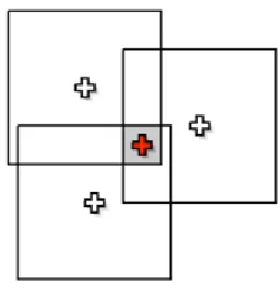
In this algorithm, each node listens to its neighbor beacon nodes and collects their position. If we consider the beacon radio radius or, the receiver node apply below algorithm signal to estimate its position.
If a beacon be in the position of (Xb, Yb), so the node estimate its position in below coordinates:
Xn є [Xb – br , Xb + br] , Yn є [Yb – br , Yb + br] (2)
[image:2.596.323.451.517.652.2]The node position is guarantees to be between the resulted squares conjunction from the above relationship with regard to the beacon radio radius. This collection is by it self a box whose maximum and minimum amounts are obtained by algorithm repetition for all the neighbor beacons of that node. At each stage, the limited new amounts are computed in ratio of the previous stage and the minimum limit is kept and at last the center part of this limit is computed and it is estimated to be the position of that node. Figure (1) represents this issue [6].
Figure .1 The original bounding box
2.1.1.2.
Using movable beacon
98
information to the nodes and of course, these nodes should beaware of this robot presence and before computation its exact location, we it for a signal from this robot. Using movable beacon means to have several beacons. So by using it, we can consider the initial beacons number less than the mentioned one [9].
Anchor– free methods
In this section, examples of anchor-free algorithms are represented.
2.2.2.1.
Spotlight [10]
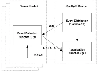
The main idea of this kind of positioning is to produce control occurrences in a ground on which the sensor nodes are spread. For example, an occurrence can be light presence in the area. By applying receive time of an occurrence by the sensor rode and the relative properties to the produced occurrence space, the information of space (e.g. position) relative to that sensor node can be obtained. System architecture for positioning the spot light model is presented in figure (2). By supporting 3 function, the positioning procedure is followed as below [10, 11].
1. In a time period, the spotlight distributes the occurrences of e (t) in the A space.
2. While occurrence distribution, the sensor nodes records receive time order of the occurrences.
[image:3.596.319.541.392.746.2]3. Spotlight device estimates the sensor node position by applying time order and known function E(t) [12].
Figure 2. The architecture of spotlight system.
3.
A NEW ALGORITHM BASED ON
COMPUTATIONAL, GEOMETRIC
In this section, a new algorithm based on computational geometry is presented and its efficiency is compared with the best range-free algorithm i.e. bunding box by performing in MATLAB software.
Definition of improved bounding box
algorithm
In the presented bounding box algorithm in the section of previous alternatives, if the number of correct positioned nodes won't be negligible, these nodes can by themselves be applied as extra beacons, that means when a node wants to estimate its own position, can use the other non beacon nodes as extra beacons which computed their position before and are placed in that node radio radius. If a node knows that it has
found its ideal position coordinates, it can operate as a beacon and start to spread its position coordinates information and its location information is included in other nodes coordinates computation. Since the radio radians of the normal nodes is smaller than the beacon ones, the node that is applied as extra beacon, will supply less positions collection, so the positioning accuracy increases significantly.
To do this performance, the present capabilities of beacon nodes are added to the normal nodes. If the node succeeded to own beacon ability, then starts to spread its position coordinates. When the other node receives this information it's essential to know that information is sent from a normal node to consider the proportional radio radius. So sent information by a normal node has estimated its own position successfully, should contain radio radius of that node in addition to the position coordinates.
Implementation
All the geometric approaches of positioning problem like an algorithm need a lot of nodes. Here, all the researches are simulated whit MATLAB model.
Having the network size and the relative density of the nodes and beacons, two networks are formed and the nodes are distributed randomly. As a complete system is made (figure 3) a rapid test guarantees that no position that contains both beacon and nodes is available, otherwise the node dislocates from the network. The positioning process is performed in every node and includes five stages:
A local network is formed arrowed the nodes position & this network is as large as radio radius. This means that a node can't recognize the beacons outside this location.
A test is carried out in beacons network, a test which lists all the heard beacons & their position in a beacon position table.
For all the listed beacons, the previously mentioned bounding box relationship is applied to decrease the position probability collections.
After passing all the beacons, if this set be equal to 1, the node can position itself successfully, otherwise the set size is kept as uncertain amount to allow the position be estimated as a center part of this collection.
The estimation network is changed and up to dated by keeping the error parameters track.
[image:3.596.53.250.402.547.2]99
When the mentioned five stages are obtained for all the sensornodes, the estimation network of the node is completed and can be compared to the initial node network.
There are several statistical to compare like the exact positioned node numbers, the average and maximum amount.
Modeling & Evaluating Tests of the New
Presented Algorithm
As soon as the network formed randomly, several specifications such as separated nodes or beacon in the corner could appear. A node on the network edge will hear less than half of heard beacons by the node placed in the middle and this cause the general efficiency to decrease. To be released of such special cases, each simulation is performed for several times (5 to 10 times) and the average amounts are obtained. Even if the network be formed by means of density amounts, the number of the nodes and beacon can have fluctuation from one simulation to another. To compare, the statistical results are mentioned as percent ones. The first simulation to evaluate the effect of the network settings (density, radio amplitude and size) is designed according to many involved parameters. There is no possibility of changing all these factors simultaneously. So the first part of this examination evaluates them as two or three parts and draws the conjunctions results.
For the bounding box algorithm presented in the section of previous alternatives and for radio amplitude presented, the estimated exact nodes ration is increased by increasing beacons density. When the beacons density for a network increases by fixed density, the radio radius enlargement allows the exact estimated nodes to increase. But after a definite distance, this operation is no longer proper. Making decision for correct radio radius is an important problem. For a network represented by 100 by 100 grid a radio radius of 16 is about the same as a radio range of 8 in a 50 by 50 network.. The only difference concerns the accuracy. The best accuracy that can be obtained equals to 1 unit.
So if the radio radius of 12 allows to 125m diffusion, then the model accuracy will be 10m. by applying the miner network, the computations will be simpler but the expense for the high accuracy increases. By this supposition that 1 unit means 10 m, the used network in this modeling will be a network with 1km2 size.
A node is positioned correctly when the algorithm manages in a such way that the maximum position difference i.e. positioning be in the dimensions of 10×10m. By having the density entry of 30% for the nodes & 8% for beacons, the network has approximately 2400 node and 770 beacons. The bounding box algorithm localizes 30 to 35% of the nodes exactly. By supposing the radio radius be 12 units, 32% is position completely. Table (1) shows that 52% is considered as false positioning. This means that 16% of the nodes could not reach to the exact positioning of 1 that is based on the computation of the center of gravity of uncertain areas.
2 - These nodes have probably a good accuracy (Perhaps 2, 3 or 4, but their amounts are not reachable in this model). The false positioned nodes in this special case represent an idea of the algorithm efficiency rate.
According to the detailed results, these nodes have mean of uncertainty zone of 13.8 units. The average height equals 3.9 units and its width equals to 3.8 We can obtain data with closer look to figure (6) and
observe that some of the
nodes have uncertainty zone greater than 100 (here the
[image:4.596.315.547.80.293.2]maximum rate is 168) and most of them have the rates
less than 20.
Figure 4. The results of bounding box.
It is obvious that 16% of the nodes could not reach to the positioning accuracy of 1 that is based on computing uncertain areas center of gravity.
In the case of new presented algorithm i.e. improved bounding box and by considering all the assumptions & the initial amount of performing previous algorithm, the results of tables performing previous algorithm, the results of tables (2), (3) could be obtained that in general case shows the presented algorithm superiority to the previous algorithms with regard to the estimation accuracy.
The expected and concerned point in this simulation is that the number of the correct estimated nodes increase by the nodes radio radius increasing. The unexpected and considerable point observed in this table is that the number of correct estimated nodes decrease by beacons radio radius increasing.
Table 1
The Obtained Accuracy Using the Bounding Box Algorithm for Radio Radius of 11 to 14.
Table 2
100
Table 3
The Obtained Accuracy Using the New Algorithm for Radio Radius of 3 to 6.
4.
CONCLUSION
The researches carried out in the field of positioning in wireless sensor networks have showed that there is no general optimized algorithm in this case. A proper algorithm should be represented depend on the position and situation e.g. the network size or distribution method. In this paper, range methods and range–free methods are discussed. range–free methods contain the methods based Implementation results in MATLAB Tool Box show that the presented algorithm has high estimation accuracy in comparison to the similar geometric algorithms. Therefore in military and civil applications, it can be the replace of costly range algorithms or the similar geometric algorithms that have less accuracy.
5.
REFERENCES
[1] D .Culler, D.Estrin and M .Strivastava, Overview of Sensor networks IEEE Computer Society, 2004.
[2] D.Gay, P.Levis, D.Culler and E.Brewer , nesC1.1 Language Reference Manual, May 2003.
[3] I.F .Akyildiz, W .Su, Y.Sankara subramaniam, and E.Cayirci, A survey On sensor networks, IEEE Communications Magazine, 2005.
[4] C. Chong and S .Kumar, Sensor Networks: Evolution, Opportunities and Challenges, Proceedings of the IEEE, August 2006.
[5] K .White house and D. Culler Micro-calibration in Sensor/Actuator Net works, UC Berkeley, 2006.
[6] S. N. Simic and S. Sastry, A distributed algorithm for localization in Random wireless networks, Discrete Applied Mathematics, UC Berkeley, November2007.
[7] Fang,L., Du,W.,and Ning,P. A beacon-less location discovery scheme for Wireless sensor networks. In IEEE Conference on Computer Communications (Infocom) 2008.
[8] He,T.,Huang ,C, Blum, B., Stank Vic ,J .A. ,and Abdelzaher ,T. Range-Free localization schemes in large scale sensor networks. In ACM International Conference on Mobile Computing and Networking (Mobicom) 2008.
[9] Neal Patwari and III Alfred O.Hero.Using proximity and quantized rss for sensor localization in wireless networks. In WSNA’03: Proceedings of the 2nd ACM international conference on Wireless sensor networks and applications, pages 20–29, NewYork, NY, USA, 2007. ACM Press.
[10]Nissanka B. Priyantha, Hari Balakrishnan, Erik Demaine, and Seth Teller, Anchor-free distributed localization in sensor networks. Technical Report 892, MIT, MIT Laboratory for Computer Science, April 2008.
[11]Nissanka B.Priyantha, Anit Chakraborty, and Hari Balakrishnan. The cricket location-support system. In MobiCom’00: Proceedings of the 6th annual international
conference on Mobile computing and networking, pages 32–43, New York, NY, USA, 2009.ACM Press.