Comparative Analysis of Software Effort Estimation
Techniques
P.K. Suri,
PhD Dean, Research and Development; Chairman,CSE/IT/MCA, HCTM Technical Campus, Kaithal,
Haryana, India
Pallavi Ranjan
HCTM Technical CampusKaithal, Haryana, India
ABSTRACT
Project Failure is the major problem undergoing nowadays as seen by software project managers. Imprecision of the estimation is the reason for this problem. As software grew in size and importance it also grew in complexity, making it very difficult to accurately predict the cost of software development. This was the dilemma in past years. The greatest pitfall of software industry was the fast changing nature of software development which has made it difficult to develop parametric models that yield high accuracy for software development in all domains. Development of useful models that accurately predict the cost of developing a software product. It is a very important objective of software industry. In this paper, several existing methods for software cost estimation are illustrated and their aspects will be discussed. This paper summarizes several classes of software cost estimation models and techniques. To achieve all these goals we implement the simulators. No single technique is best for all situations, and that a careful comparison of the results of several approaches is most likely to produce realistic estimates.
General Terms
Software Estimation Techniques, Simulation
Keywords
Simulation, Delphi, Effort Estimation, COCOMO
1.
INTRODUCTION
Software engineering cost (and schedule) models and estimation techniques are used for a number of purposes [1]. These include:
Budgeting
Tradeoff and risk analysis Project planning and control
Software improvement investment analysis
1.1 Need of Software Effort Estimation
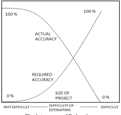
Small Projects are very easy to estimate and accuracy is not very important. But as the size of project increases, required accuracy is not very important. But as the size of project increases, required accuracy is very important which is very hard to estimate. A good estimate should have amount of granularity so it can be explained. Since the effort invested in a project is one of the most important and most analyzed variables. So the prediction of this value while we start the software projects, it helps to plan any forthcoming activities
[image:1.595.329.531.281.473.2]adequately. Estimating the effort with a large value of reliability is a problem which has not been solved yet.
Fig. 1 Accuracy of Estimating
1.2 Simulation
Simulation is defined as a process of designing model of a real system and conducting experiments with this model for the purpose either of understanding the behavior of the system or evaluating various strategies within the limits imposed by a criterion or a set of criteria for the operation of the system. Once a simulation is in use, running it on new data or with new parameters is usually just a matter of few keystrokes or dragging and dropping a different life. Depending upon the variables being deterministic or random, the simulation models can be classified as
1. Deterministic Simulation 2. Stochastic Simulation
the system in its simulated environment. A system that relies heavily upon random behavior is referred to as stochastic system.
Problem Solving using Simulation
The application of Simulation involves specific steps in order for the simulation study to be successful. Regardless of the type of problem and objective of the study, the process by which the simulation is performed remains constant. The following steps describe the problem solving using simulation:
1. Problem Definition: The initial step involves the goals of the study and determining what needs to be solved. The problem is further defined through objective observations of the process to be studied. Care should be taken to determine whether simulation is the appropriate tool for the problem under investigation.
2. Project Planning: The tasks for completing the project are broken down into work packages with a responsible party assigned to each package. Milestones are indicated for tracking progress. This schedule is necessary to determine if sufficient time and resources are available for completion.
3. System Definitions: This step involves identifying the system components to be modeled and the performance measures to be analyzed. Often the system is very complex, thus defining the system requires an experienced simulator who can find the appropriate level of detail and flexibility.
4. Modern Formulations: Understanding how the actual system behaves and determining the basic requirements of the model are necessary in developing the right model. Creating a flowchart of how the system operates facilities the understanding of what variables are involved and how these variables interact.
5. Input Data collection and analysis: After formulating the model, the type of data to collect is determined. New data is collected and/or existing data is gathered. Data is fitted to theoretical distributions. For example, the arrival rate of a specific part to the manufacturing plant may follow a normal distribution curve.
6. Model Translations: The model is translated into programming language. Choices range from general purpose languages to simulation programs.
7. Verification and Validation: Verification is the process of ensuring that the model behaves as intended, usually by debugging or through animation. Verification is necessary but not sufficient for validation, i.e. a model may be verified but not valid. Validation ensures that no significant difference exists between the model and the real system.
8. Experimentation and Analysis: Experimentation involves developing the alternative model(s), executing the simulation runs, and statistically comparing the alternative(s) system performance with that of the real system.
9. Documentation and Implementation: Documentation consists of the written report the required steps of a simulation study establishes the likelihood of the study’s success. Although knowing the basic steps in the simulation study is important, it is equally important to realize that not very problem should be solved using simulation.
1.3
Current
Trends
in
Software
Development
Prior 1970, estimation of effort was done manually by using Thumb rules or some algorithms which were based on Trial and error[10].
1970 was an important period to predict the costs and schedules for software development. Automated Software cost estimating tools were built. Some difficulties were experienced building large software systems [17].
During early 1970’s the first automated software estimation tool had been built. The prototyping composite model is COCOMO (Constructive Cost Model) developed by Barry Boehm and is described in book Software Engineering Economics [10]. 1975, Function Point Analysis for estimating the
size and development effort. This metric was based on five different attributes [2]
Inputs
Outputs
Inquires
Logical Files
Interfaces
1977, PRICE-S Software estimation model was designed by Frank Freiman. It was the commercial tool to be marketed in United States.
1979, SLIM (Software Life Cycle Model) was introduced to US-Market by Lawrence H. Putnam based on Norden Rayleigh Curve [28].
1980, The U.S. Department of Defense (DoD) introduced Ada programming language in 1983 and it reduced the cost of developing large systems. That model was named as Ada-COCOMO [29]. 1981, Dr. Barry Boehm released his book “Software
Engineering Economics” in which he highlighted the essential algorithms of Constructive Cost Model (COCOMO). Allan Albrecht published an article to the FPA method. This article sharpened the rules for rating the complexity of software [10].
1982, Tom deMarco imparted a book “controlling software projects” in which he introduced a functional metric that inherited some of the features of Albrecht’s function point, but was developed independently.
1983, Charles Symons, a British software estimating researcher, he introduced Mark II function point metric [13].
1984, IBM done a major revision of his function point metric which is basis of today’s function points [10].
1985, Caper Jones extended the concept of Function Point to include the effect of computationally complex algorithms [3].
1986, IFPUG (International Function Point Users Group) was founded in Toronto, Canada due to rapidly growing usage of Function Point Metrics. 1990, Barry Boehm, at university of Southern
California began to revise and extend the concept of original COCOMO model.
1992, Betteridge, R. worked on software costing. There was a method called Mark II Function Point which predicted cost of number of projects [9]. 1993, the new version of COCOMO was introduced
called COCOMO 2.0 which emerged in 1994[8]. 1994, Rajiv D Banker and Hsihui Chang and Chris
F Kemerer, they found it useful for cost estimation and productivity evaluation purposes’ to think of software development as an economic production process [4].
1996, Sophie Cockroft, obtained accurate size estimations from the early system specifications [15].
1997, Existing models were reviewed and more focus was on accuracy.
1998, Chatzoglou constructed a new model called MARCS to give predictions of the resources (time, effort, cost, people) [14].
1999, J. J. Dolado, He made a research about the estimation using the technique of Genetic Programming (GP) for exploring possible cost functions [16].
2001, A new approach was proposed based on reasoning by analogy and linguistic quantifiers were used to estimate the effort [1].
2002, M.Jorgensen, expert estimation was the most frequently applied estimation strategy for software projects [20].
2003, Yunsik Ahn, Jungseok Suh, Seungryeol Kim and Hyunsoo Kim, they discussed software maintenance and proposed SMPEEM (Software Maintenance Project Effort Estimation) [34]. 2004, There were surveys that potentially lead to
low data quality. The idea of EBSE (Evidence based Software Engineering) was proposed by Barbara [5].
2005, There was sequence which was decided and needed to be carried out for software estimation Sizing Project deliverables, Estimating quality and defect Removal efficiency, Selecting Project activities, Estimating staffing levels, Estimating Effort, Estimating Costs, Estimating Schedules, Estimating requirements growth during development [12].
2006, Stein Grimstad, effort estimate was frequently used without sufficient clarification of its meaning, and that estimation accuracy is often evaluated without ensuring that the estimated and actual effort were comparable [32].
2007, Different methods were introduced for estimating the effort. The average accuracy of expert judgment based effort estimates were higher than the average accuracy of models [21].
2008, Parvinder S. Sandhu, He focused on predicting the accuracy of models. As Neuro-Fuzzy system was able to approximate the non-linear function with more precision. So, neuro-fuzzy system was used as a soft computing approach to generate the model [26].
2009, During this year, some theoretical problems were identified that compared estimation models. It was invalid to select one or two datasets to prove validity of a new technique [6].
2010, Different estimation techniques were combined to reduce the error and keep control over the deviation of estimates away from actual [33,24].
2011, Many estimation techniques were proposed and used extensively by practitioners for use in Function Oriented Software development [31]. 2012, There were many software size and effort
measurement methods proposed in literature, they were not widely adopted in practice. A lot of commercial software costs estimating tools have been released till today [18].
2.
SOFTWARE ESTIMATION
Project Manager must know the effort, schedule and functionality in advance. Project factors change in the duration of a project, and they may change a lot. The main thing is to predict the factor by which they change [10]. So the process of estimation needs to be carried out. Estimating is the process of forecasting or approximating the time and cost of completing project deliverables or The task of balancing the expectations of stakeholders and the need for control while the project is implemented.
Significant Research was carried out by Boehm in software cost modeling which began with the extensive 1965 study of the 105 attributes of 169 software project. This led to some useful partial models in the late 1960s and early 1970s. Although much work was carried on developing models of cost estimation, all of them were in same dilemma: “It was very difficult to predict the accurate cost of software development as software grew in size and importance it also grew in complexity.” The fast changing nature of software development has made it very difficult to develop parametric models that yield high accuracy for software development in all domains. Software development costs continue to increase and practitioners continually express their concerns over their ability to predict accurately the costs involved. This was a major pitfall experienced. Development of useful models that constructively explain the development life-cycle and accurately predict the cost of developing a software product was a major objective. Hence, many software estimation models have been evolved.
Figure 2 lists a number of examples of estimation techniques. These are classified into the following categories.
2.1 Estimation by Analogy
It means creating estimates for new projects by comparing the new projects to similar projects from the past. As the algorithmic techniques have a disadvantage of the need to calibrate the model. So, the alternative approach is “analogy by estimation”. But it requires considerable amount of computation. This process is much simple. But not all organizations have historical data to satisfactorily use analogy as means of estimation. ISBSG (International Software benchmarking Standards Group) maintains and exploits a repository of International Software Project Metrics to help software and IT business customers with project estimation; risk analysis, productivity, and benchmarking [22].
2.2 Expert Opinion
Fig. 2 Software Estimation Techniques
2.2.1 Delphi
Delphi is a place in Greece, which was supposed to confer predictive powers to person. A temple was built there and virgin girls were appointed there to answer questions about the future, they were called oracles. Oracle’s prophecies were considered prophetic or at least wise counsel [23]. So, Delphi technique was derived from them. Under this method, project specifications are given to a few experts and their opinion taken. Steps:
1. Selection of Experts. 2. Briefing to the Experts
3. Collation of estimates from experts 4. Convergence of estimates and finalization
Selection of Experts: Experts are selected who have software development experience, who have worked and possess knowledge in application domain at hand, they may be from within or without the organization.
Briefing the Experts: The experts need to be briefed about the project. They need to know the objectives of estimation, explanation of project scope, completion and its nature in project bidding. Collation of estimates received from experts: The experts are expected to give one figure for the development effort and optionally software size.. Each oracle gives the opinion.
Name of Expert Size Effort
Expert 1 A X
Expert 2 B Y
Expert 3 C Z
…. …. ….
Expert n K L
Convergence of estimates and finalization: Now the estimates are converged using either the statistical mode from opinions offered by experts or extreme estimates are interchanged i.e. higher estimate is given to expert who gave lowest figure estimate, lower estimate is given to expert who gave highest figure estimate, average estimate can be derived using arithmetical average.
T(e)={t(o)+4t(m)+t(p)}/6 Var2={t(p)-t(o)}2/36
Fig.3 Delphi Estimation
2.3 Putnam’s Software Life-cycle Model
(SLIM)
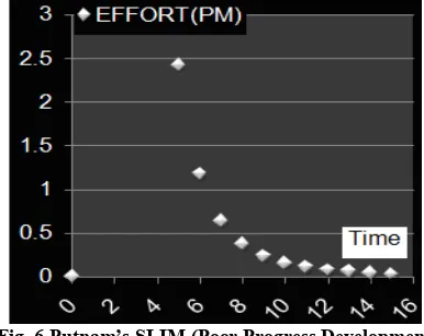
[image:4.595.49.288.571.636.2]The Putnam Model is an empirical software effort estimation model [36, 27]. Lawrence H. Putnam in 1978 [28] is seen as pioneering work in field of Software Process Modeling. This model describes the time and effort required for a project of specified size. SLIM (Software Lifecycle Management) is name given by Putnam. Closely related software parametric models are COCOMO (Constructive Cost Model), PRICE-S (Parametric review of Information for Costing and Evaluation Software) and (SEER-SEM) Software Evaluation and Estimation of Resources- Software estimating model.
[image:4.595.328.529.595.738.2]Fig. 5 Rayleigh’s Distribution (Good Progress Development c=4000)
Nordon studied the staffing patterns of several R & D projects. He noted that the staffing pattern can be approximated by a Rayleigh distribution curve. Putnam studied the work of Nordon and determined that Rayleigh curve can be used to relate the number of lines of code to estimate time and effort required by project.
4/3 d 1/3 k
K
t
C
L
where L is the product size. C
k is the state of technology
constant which shows the progress of programmer. K is the total effort. Td is the time required for system to complete the
software. Ck =2 which means poor progress environment- no
methodology, poor document, poor review etc. Ck =8 implies
good software development. Ck=11 means excellent
development- automated tools and techniques are used. The value of Ck can be computed using historical data of an
[image:5.595.323.533.85.216.2]organization.
[image:5.595.69.262.416.569.2]Fig. 6 Putnam’s SLIM (Poor Progress Development c=7000)
Fig. 7 Putnam’s SLIM (Good Progress Development c=25000)
Fig. 8 Putnam’s SLIM (Excellent Progress Development c=40000)
2.4 COCOMO
The Constructive Cost Model (COCOMO) was launched in 1981 by Barry Boehm. It is also called COCOMO 81. The model assumes that the size of a project can be estimated in thousands of delivered source instruction and then uses a non-linear equation to determine the effort for the project. COCOMO II is the successor of COCOMO 81 and is better suited for estimating modern software development projects and updated project database. The need for the new model came as software development technology moved from mainframe and overnight batch processing to desktop development, code reusability and the use of off-the-shelf software components.
COCOMO consists of a hierarchy of three increasingly detailed and accurate forms. The first level, Basic COCOMO is good for quick, early, rough order of magnitude estimates of software costs, but its accuracy is limited due to its lack of factors to account for difference in project attributes (Cost Drivers). Intermediate COCOMO takes these Cost Drivers into account and Detailed COCOMO additionally accounts for the influence of individual project phases.
2.4.1 Basic COCOMO
Basic COCOMO computes software development effort (and cost) as a function of program size. Program size is expressed in estimated thousands of source lines of code (SLOC). COCOMO applies to three classes of software projects:
Organic projects - "small" teams with "good" experience working with "less than rigid" requirements
Semi-detached projects - "medium" teams with mixed experience working with a mix of rigid and less than rigid requirements
Embedded projects - developed within a set of "tight" constraints. It is also combination of organic and semi-detached projects.(hardware, software, operational, ...)
The basic COCOMO equations take the form
E/D
P
d
*
c
D
b
*
a
E
b b
b b
[image:5.595.70.263.599.743.2]Effort Applied (E) = (KLOC)*[ man-months ]
Development Time = (Effort Applied)* [months]
People required (P) = Effort Applied / Development Time [count]
where, KLOC is the estimated number of delivered lines (expressed in thousands ) of code for project. The coefficients ab, bb, cb and db are given in the following table:
Software project ab bb cb db
Organic 2.4 1.05 2.5 0.38
Semi-detached 3.0 1.12 2.5 0.35
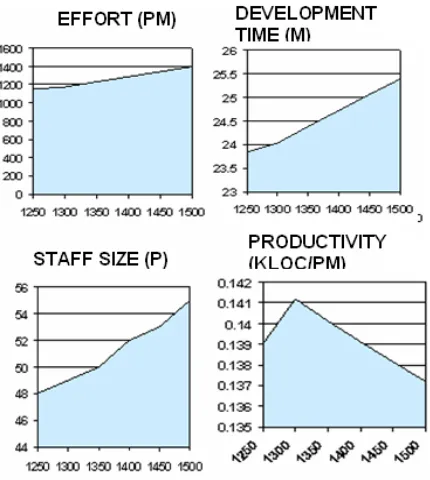
[image:6.595.327.531.75.262.2]Embedded 3.6 1.20 2.5 0.32
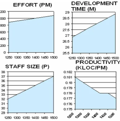
Fig. 9 Organic Project(C Multiplication Factor= 128 LOC/FP)
[image:6.595.60.270.186.486.2]Fig. 10 Semidetached Project (C Multiplication Factor= 128 LOC/FP)
Fig. 11 Embedded Project (C Multiplication Factor= 128 LOC/FP)
2.4.2 Intermediate COCOMOs
Intermediate COCOMO computes software development effort as function of program size and a set of "cost drivers" that include subjective assessment of product, hardware, personnel and project attributes. This extension considers a set of four "cost drivers", each with a number of subsidiary attributes:-
[image:6.595.331.522.447.686.2] Hardware attributes Personnel attributes Project attributes Product attributes
[image:6.595.67.261.529.724.2]Fig. 13 Semidetached Project (C Multiplication Factor= 128 LOC/FP)
Fig. 14 Embedded Project (C Multiplication Factor= 128 LOC/FP)
3.
CONCLUSION and FUTURE WORK
If the estimation is done accurately, it results in error decrease. Estimation process reflects the reality of project’s progress. It avoids cost/budget or schedule overruns. This process is quite simple which takes a few inputs. This assessment framework helps inexperienced team improve project tracking and estimation. Much work can be carried on it. Various COCOMO parameters can be adjusted. Further work can be carried on learning based methods which apply weights to calculation of each software module based on
priorities and criticalities. Tool development is currently in progress. A good estimate should have amount of granularity so it can be explained. Since the effort invested in a project is one of the most important and most analyzed variables.
4. ACKNOWLEDGMENTS
Sincere Thanks to HCTM Technical Campus Management Kaithal- 136027, Haryana, India for their constant encouragement.
5.
REFERENCES
[1] Ali Idri, Alain Abran, Taghi M. Khosgoftaar. 2001. Fuzzy Analogy- A New Approach for Software Cost Estimation. International Workshop on Software Measurement (IWSM’01).
[2] Allan J. Alberecht and John E. Gaffhey, November 1983, Software Function, Source Lines of Code and Development Effort Prediction : A software Science Validation . IEEE transactions on Software Engineering.
[3] Allan J. Alberecht, May 1984. AD/M Productivity Measurement and Estimation Validation, IBM Corporate Information Systems. IBM Corp.
[4] Banker, R. D., H. Chang, et al. (1994). "Evidence on economies of scale in software development." Information and Software Technology 36(5): 275-282.
[5] Barbara A. Kitchenham, Tore Dybå, Magne Jørgensen. 2004. IEEE Proceedings of the 26th International Conference on Software Engineering (ICSE’04)
[6] Barbara Kitchenham, Emilia Mendes. 2009. Why Comparative Effort Prediction Studies may be Invalid © ACM 2009 ISBN: 978-1-60558-634-2.
[7] Barry Boehm, Chris Abts and Sunita Chulani. 2000 Software development cost estimation approaches. A survey. Annals of Software Engineering.
[8] Barry W. Boehm, Bradford dark, Ellis Horowitz, Chris Westland, Ray Madachy and Richard Selby. Cost Models for Future Software Lifecycle Processes: COCOMO 2.0 Annals of Software Engineering. Volume 1,pp,57-94,1995. An earlier description was presented in the tutorial “COCOMO, Ada COCOMO and COCOMO 2.0” by Barry Boehm in the Proceedings of Ninth International COCOMO Estimation Meeting. Los Angeles, CA, 6-7 October 1994.
[9] Bergeron, F. and J. Y. St-Arnaud (1992). "Estimation of information systems development efforts: a pilot study." Information and Management 22(4): 239-254.
[10] Boehm, 1981 “Software Engineering Economics”, Prentice Hall.
[11] Boehm, B. W. and P. N. Papaccio (1988). Understanding and controlling software costs. IEEE Transactions on Software Engineering 14(10): 1462-1477.
[12] Capers Jones, Chief Scientist Emeritus Software Productivity Research LLC. Version 5 – February 27, 2005. How Software Estimation Tools Work.
[13] Charles Symons 1991. Software Sizing and Estimation Mark II function Points (Function Point Analysis), Wiley 1991.
[image:7.595.59.274.362.602.2]prediction models." Automated Software Engineering 5(2): 211-243.
[15]Cockcroft, S. (1996). "Estimating CASE development size from outline specifications." Information and Software Technology 38(6): 391-399.
[16]Dolado, J. J. (2000). "A validation of the component-based method for software size estimation." IEEE Transactions on Software Engineering 26(10): 1006-1021
[17]F.Brooks, The Mythical Man-Month; Essays on Software Engineering, 1975. Addison-Wesley, Reading, Massachusetts.
[18]Jovan Popović1 and Dragan Bojić1. 2012. A Comparative Evaluation of Effort Estimation Methods in the Software Life Cycle. ComSIS Vol. 9, No. 1, January 2012
[19]Lawrence H. Putnam 1978. A General Empirical Solution to the Macro Software Sizing and Estimation problem. IEEE transactions on Software Engineering.
[20]Magne Jørgensen, A Review of Studies on Expert Estimation of Software Development Effort, March 2002.
[21]Magne Jørgensen. May 2007 Forecasting of Software Development Work Effort: Evidence on Expert Judgment and Formal Model.
[22]Martin Shepperd and Chris Schofield, Barbara Kitchenham, 1996.Effort Estimation Using Analogy. IEEE Proceedings of ICSE-18
[23]Murali Chemuturi, Delphi Technique for software estimation
[24]M. V. Deshpande, S. G. Bhirud. August 2010. Analysis of Combining Software Estimation Techniques. International Journal of Computer Applications (0975 – 8887)
[25]Narsingh Deo, System Simulation with Digital Computer. Prentice Hall of India Private Limited.
[26]Parvinder S. Sandhu, Porush Bassi, and Amanpreet Singh Brar. 2008. Software Effort Estimation Using Soft Computing Techniques. World Academy of Science, Engineering and Technology 46 2008.
[27]Putnam, Lawrence H.; Ware Myers (2003). Five core metrics : the intelligence behind successful software management. Dorset House Publishing. ISBN 0-932633-55-2.
[28]Putnam, Lawrence H. (1978). "A General Empirical Solution to the Macro Software Sizing and Estimating Problem".IEEE transactions on Software Engineering, VOL. SE-4, NO. 4, pp 345-361.
[29]Robert C. Tausworthe, 1981. Deep Space Network Estimation Model, Jet Propulsion Report.
[30]Rolf Hintermann 2002/2003 Seminar on Software Cost Estimation. Introduction on Software Cost Estimation. Institut für Informatik der Universität Zürich.
[31] Samaresh Mishra1, Kabita Hazra2, and Rajib Mall3. October 2011. A Survey of Metrics for Software Development Effort Estimation. International Journal of Research and Reviews in Computer Science (IJRRCS)
[32] Stein Grimstad*, Magne Jørgensen, Kjetil Moløkken-Østvold. 13 June 2005. Software effort estimation terminology: The tower of Babel. Information and Software Technology 48 (2006) 302–310
[33] Vahid Khatibi, Dayang N. A. Jawawi. 2010. Software Cost Estimation Methods: A Review. Journal of Emerging Trends in Computing and Information Science.
[34] Yunsik Ahn, Jungseok Suh, Seungryeol Kim and Hyunsoo Kim. July 2002. Journal of Software Maintainence and Evolution : Research and Practice.
6.
AUTHORS PROFILE
Prof. P.K.Suri, Dean (R & D), Chairman & Professor (CSE/IT/MCA) of HCTM Technical Campus, Kaithal, since Nov. 01, 2012 . He obtained his Ph.D degree from Faculty of Engineering, Kurukshetra University, Kurukshetra and Master’s degree from IIT Roorkee (formerly . He started his research carrier from CSIR Research Scholars, AIIMS. He worked former as a dean Faculty of Engineering & Technology, Kurukshetra University, Kurukshetra, Dean Faculty of Science, KUK, Professor & Chairman of Department of Computer Sc. & Applications, KUK. He has approx 40 yrs experience in different universities like KUK, Bharakhtala University Bhopal & Haryana Agricultural university , Hissar. He has supervised 18 Ph.D. students in Computer Science and 06 students are working under his supervision. Their students are working as session judge, director & chairpersons of different institute. He has around 150 publications in International/National Journals and Conferences. He is recipient of 'THE GEORGE OOMAN MEMORIAL PRIZE' for the year 1991-92 and a RESEARCH AWARD –“The Certificate of Merit – 2000”for the paper entitled ESMD – An Expert System for Medical Diagnosis from INSTITUTION OF ENGINEERS, INDIA. The Board of Directors, governing Board Of editors & publication board of American Biographical institute recognized him with an honorary appointment to Research board of Advisors in 1999. M.P. Council of Science and Technology identified him as one of the expert to act as Judge to evaluate the quality of papers in the fields of Mathematics/Computer Science/ Statistics and their presentations for M. P. Young Scientist award in Nov. 1999 and March 2003. His teaching and research activities include Simulation and Modeling, Software Risk Management, Software Reliability, Software testing & Software Engineering processes, Temporal Databases, Ad hoc Networks, Grid Computing, and Biomechanics.