Real and financial sector interaction under liberalisation in an open developing economy

Munich Personal RePEc Archive

Real and financial sector interaction

under liberalisation in an open

developing economy

Goyal, Ashima and Dash, Shridhar

Indira Gandhi Institute of Development Research

August 2000

Online at

https://mpra.ub.uni-muenchen.de/23966/

Preprint from Meteroeconomica, 51, 3, 257-283, 2000.

Real and financial sector interaction under liberalisation in an open

developing economy

Ashima Goyal* and Shridhar Dash

Associate Professor, Indira Gandhi Institute of Development Research Assistant Manager, GE Capital Markets

Abstract

A short-run model incorporates instantaneous portfolio equilibrium with macroeconomic flows to clarify the structure of real-financial sector interactions. If equity and foreign exchange markets are introduced in structuralist theories of asset markets in developing countries, the key result that a fall in money supply raises the rate of inflation now holds only under special conditions on partial derivatives. But there is a tendency for interest rates to rise and for fluctuations in asset prices. Fuller integration of asset markets moderates these fluctuations. Outcomes are stable in spite of the generalized complementarity distinguishing equity markets from loan markets. Expectations play a major role. Implications for policy are to link domestic interest rates to foreign, remove artificial barriers to market integration, and stimulate demand as well as supply.

Acknowledgement

The paper was presented at the IGIDR Conference on Money and Finance, December 1998. We thank the audience for stimulating questions. Prakash Apte, Sunil Ashra, Basudeb Guha-Khasnobis, Raghbendra Jha, Ganti Subramanyam and a referee of this journal gave useful comments.

Keywords: real-financial, portfolio, excess demands, volatility, saddle-stability.

JEL Classification: E44, O11

1. Introduction

A well-known result1 in the structuralist literature is that in an underdeveloped

financially repressed economy, monetary contraction can cause inflation due to a rise in

working capital costs. We show how this result is modified in a world in which the rate of

inflation clears goods markets and equity markets are present with a market-clearing rate

of return. Although the standard result holds only under special conditions, it is

re-instated when equity markets become more active. From the eighties onwards, financial

reform, opening out and inflows of foreign capital have characterized many developing

countries. Adapting the structuralist model to incorporate these features is useful to

clarify the structure of real-financial sector interactions. The analysis points to the

importance of a monetary policy that prevents rise and fluctuations in interest rates.

Ours is a very short-run model that incorporates instantaneous portfolio

equilibrium with macroeconomic flows. The focus is on daily variations in asset prices.

Output and the price level are fixed at this horizon. But forward looking inflation

expectations clear the goods market2. Since inflation affects returns to assets, and

inflationary expectations can match the speed of asset price adjustment, the endogenous

variables, at this time horizon, are the rate of inflation, the interest rate and equity returns.

Over a longer time period, these prices would influence the evolution of output.

Expectations lead to the jumps in asset prices that clear markets. As administrative

controls are removed, expectations are more freely reflected in prices. In arbitrage across

assets, the generic assumption made is that asset price elasticities exceed quantity

elasticities, because price expectations act as jump variables.

Since both the demand and supply side of the goods market are modelled, the

interest rate can affect inflation through cost-push. If the negative effect of the interest

rate on goods market supply exceeds its negative effect on demand, a rise in inflation

would be required to clear the goods market after a rise in interest rates. Profit rates rise

with inflation and fall with interest rates and through these deeper determinants influence

both goods market demand and equity returns.

Equity markets are distinguished from loan markets by generalized

complementarity, in the sense that a rise in stock returns increases excess demand in all

markets. The reason equity is risky compared to debt is that a rise in its price does not

reduce demand, so that a sustained rise or fall in equity prices is possible. Fundamentals,

such as profit rates, influence equity returns, but speculative bubbles are possible, and

these feed into excess demand in the goods market. In spite of this, it turns out that a rise

in the diversity of assets available improves stability, provided monetary policy maintains

stable interest rates.

We show that under monetary tightening during reform the rate of inflation may

fall for a range of parameter values, but there can be large fluctuations in interest rates

and equity returns. Over the medium-term this would harm output. Integration of

financial markets moderates the fluctuations. If equity markets become more important,

the structuralist result of inflation and interest rates rising together is re-established. Other

results are that the stimulus to demand must exceed that to supply in order to lower

inflation. Therefore the best policy combination is one that keeps market determined

interest rates close to world rates, stimulates demand, supply, and integration of financial

markets. Preliminary analysis of data from the Indian liberalisation supports the

theoretical hypotheses.

The structure of the paper is as follows: in section 2 a financial balance sheet is

presented and excess demands derived for the individual markets. Section 3 sets out the

key assumptions and then examines the existence and stability of equilibria. Comparative

static results are derived in section 4. Section 6 concludes. Algebraic analysis of shocks is

in the Appendix.

2. The Model

We consider excess demand functions for six markets, one real and the other financial:

the goods, loan, equity, bullion, foreign exchange and money markets. By Walras Law it

is sufficient to analyze market clearing for five markets. The financial balance sheet of

the economy represents the links between the six markets. This level of disaggregation

captures relevant distinctions in the attributes of assets such as liquid (money), fixed

income (debt), and risky (equity) assets. In addition, traditional assets (bullion) play a

major role in developing countries, and foreign exchange is acquiring importance as an

Maximisation over primitives such as technology, preferences delivers household

portfolio demand functions in a general equilibrium framework. But it is not yet possible

to derive similar qualitative restriction on signs of excess demand functions that include

asset-demands from firms. There are fundamental problems in aggregating over debt and

equity for a representative firm. Theory, such as principal-agent frameworks in

incomplete capital markets and empirical evidence support our sign restrictions. But in

order to side-step the deep problems of aggregation that affect atomistic optimising

models, we use generalised demand and supply functions that can distinguish between

supply and demand for assets from firms, households and government. A firm demands

loans and supplies equity.

After a brief discussion of the balance sheet, agents and adding up conditions

involved, we specify each of the market equilibrium conditions.

2.1 The Financial Balance Sheet: Agents and their activities

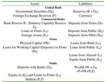
The balance sheet for the macroeconomy (table 1) reflects the financial structure of

typical reforming developing economy. Households make a portfolio choice among bank

deposits Dp; loans to firms Lp; equity of firms EP; and bullion PzZ. Bullion stock is Z, and

its price is Pz. Bullion is a generic term for unproductive assets. Households cannot hold

foreign currency or assets, or government securities Gb. After cancelling items appearing

on both sides of the balance sheet, wealth (W) is sum of high-powered money, H, value

of capital stock and bullion.

GR are government securities held by the central bank. H, equals central bank

liabilities such as currency, backed by central bank assets such as GR and foreign reserves

F. The central bank also performs the functions of a treasury, managing government debt.

Banks are the financial intermediaries that, along with households, make finance

available to firms and the government. Commercial banks hold assets in the form of

reserves comprising deposits with the central bank, R, and government securities, Gb;

loan to firms, Lb; and foreign assets, Fb. The assets are created, in order to maximise

profits, out of liabilities that consist of deposits from households, Dp; firms, Df; and non-

resident nationals (NRNs), DN. Assets must equal liabilities for each entity, therefore for

b b b N

P

f D D R L G F

D + + = + + + (1)

Commercial banks are required to hold a proportion of government securities (Gb) as

statutory liquidity ratio (SLR) requirements, but they are free to hold excess. Similarly R

can exceed the compulsory reserve ratio (CRR), but cannot fall below that. The

government deficit, GD, minus its monetization, ΔGR, determines the supply of

government securities, Gb, since:

b

R G

G

GD=Δ +Δ (2)

The treasury-bill rate, it, clears the market for these securities. Banks are allowed to hold

foreign exchange assets (Fb).

Table 1: Financial Balance Sheet

Assets Liabilities Central Bank

Government Securities (GR) Reserves (R + Gb)

Foreign Exchange Reserves (F) Currency

Commercial Banks Bank Reserve R, Statutory Liquidity Reserve

Gb

Deposits from Firms (Df)

Loans to Firms (Lb) Deposits from Public (Dp)

Foreign Assets (Fb) Deposits from NRIs (DN)

Firms

Physical Capital (PK) Loans from Bank (Lb)

Loans for Working Capital (Deposits) to Firms (Df)

Loans from Public (Lp)

Loans from Abroad (Lf)

Equity from Public (Ep)

Public

Deposits with Banks (Dp) Wealth (W = GR

+F+PK+PzZ)

Equity in (Ep) and Loans to Firms (Lp)

Firms maximise profits and raise money to finance capital accumulation (PK) and

working capital (Df) by taking loans from banks, households or foreigners. They can also

issue equity to households. The nominal rates of return are, interest rate on loans to firms,

i, rate of return on equity, ie, and on bullion: πz. The latter is the rate of bullion-price rise.

Actual inflation, π equals inflationary expectations (πe). Expectations are forward

looking. Subtracting the inflation rate from the nominal rates of return gives the real rate

of return of the assets. Since households do not hold foreign assets, they allocate wealth

(W) in a portfolio of four assets, viz. loans to firms, equity, bullion and bank deposits.

W y i i i f

L_{P 1}( , _e, _Z, _d, , )

+ − − − −

+ π π

= (3)

W y i i i f

E_{p 2}( , _e, _Z, _d, , )

+ − − − +

− π π

= (4)

W y i i i f

Z ₃( , _e, _Z, _d, , )

+ − − + −

− π π

= (5)

W y i i i f

D_{P 4}( , _e, _Z, _d, , )

+ − + − −

− π π

= (6)

Standard assumptions are made: unit wealth elasticity, positive own interest rate elasticity

i.e., f₁₁ >0, f₂₂ >0, f₃₃ >0, f₄₄ >0, and gross substitutability between assets i.e.

... 0 ,

0 ,

0 ,

0 ,

0 ,

0 _{13 21 23 31 32}

12 < f < f < f < f < f <

f By the adding up condition for

wealth3, the demand for bank deposits, which is also the demand for money can be

derived from the other three. The public keeps a fraction, f4 =DP /W, of its wealth in

the form of bank deposits. The interest rate id paid on bank deposits is administered; it

does vary in response to market pressures, but is fixed in the short-run. Firms pay the

same interest rates i to both banks and the public for their loans. Note that all these are

simplifying assumptions. Public and bank loan rates for firms may follow each other

Households hold four assets, but markets have to clear for the five assets in our

model, and the goods market. The portfolio decision gives the households’ demand for

these assets, but their supply also depends on profit maximising by firms and banks,

arbitrage by foreign capital investors, and the government deficit. The market for bank

loans clears by the adjustment in i, and equity market by ie.

2.2 The markets

Structural features allow a simplified treatment of the bullion and foreign currency

markets. The money market clears by Walras law once all other demands and supplies

are satisfied. Given the household’s portfolio decision, the demand for money balances is

determined residually from the wealth identity, and is automatically equalled to supply.

The loan market is examined in some detail and reduced form excess demand functions

are derived. It is shown that under liberalisation there is a tendency for the loan rate of

interest to rise. Excess demand functions are also derived for the equity and goods

markets. The simultaneous interaction of the last three is then examined analytically in

section 3.

The Bullion market:

After liberalisation πz follows the international price of bullion, and becomes exogenous

for a small country. In the short-run, bullion purchase is driven, not by portfolio

considerations but by consumption demands or habit persistence. Therefore we can

assume that the cross price elasticities of bullion demand are low and can be neglected.

Bullion demand is a function of income, and that is exogenous in the time horizon of our

model4.

The External Market:

We assume a managed float. Therefore, in the short-run, the exchange rate is fixed. But

banks and foreign investors can arbitrage in money markets, NRN deposits are freely

convertible, and firms can raise money abroad. Therefore a discrepancy between

domestic and foreign interest rates must be reflected in an expected depreciation or

parity holds as in equation 7, where i is the interest rate, i*is the world interest rate and εe

is the expected rate of depreciation of domestic currency.

e

i

i= * +ε (7)

If there is a monetary shock so that i rises above i*, the foreign inflow that results will be

moderated by a rise in εe. Similarly, if there is a shock in the foreign exchange market

such as a rise in the equilibrium exchange rate or in i*, the equilibrating rise in i as

arbitrage shrinks the supply of loans, may result in a further a rise in εe. Capital flows are

mobile and respond to disequilibrium, but the elasticity of asset price adjustment exceeds

that of quantity adjustment.

The loan market:

Firms have the option of borrowing abroad, therefore the demand for bank loans is:

) ; , ,

( *

+ + +

− π

=l i i i

L_bd _{b e} (8)

The demand for domestic loans falls with the interest rate, rises with world interest rate or

cost of alternative sources of funds, and with the inflation rate. Even if a rise in ie

stimulates firms to issue more equity, there is a complementary demand for more loan

finance.

To determine the supply of bank loans to firms (we assume households do not

borrow from banks), we represent the banks’ portfolio balance as follows:

1

= + + + +

+ +

=rD gbD lbD fbD and r gb lb fb

D (9)

Where r is the proportion of assets (deposits) held as reserve, gb is the proportion of

assets held as government securities, lbis the proportion of assets held as loans to firms,

and fbis the proportion of assets held as foreign assets. The total deposits (D) are

above. The loan supply available to firms from banks will be DP +DN −rD−gbD− fbD.

The portfolio decision of households decides Dp. Excess demand equilibrium for loans

then is: W f i i D f i i i G i i i R i i i D W f l EL b t b t d N b ) ( )]} ; , ( ) ; , , ( ) ; , , ( [ ) ; , , ( ) ( { ) ( 1 4 ⋅ − + + − + ⋅ − ⋅ = + ∗ − − ∗ + + − ∗ + − − ∗ − − (10)

Reforms and the interest rate: With liberalisation, the growth of money supply is

unchanged under nominal money supply targeting. But as capital inflows rise and there is

a persistent government deficit, it must be that ΔF =ΔG_R such that R and H are

constant5. GR falls to keep high-powered money, H, constant as foreign inflows increase.

The central bank sterilises capital inflows by swapping government debt for foreign

assets. This is achieved as the central bank sells government treasury bills. The treasury

bill rate (it) is no longer administered and adjusts to clear the market for government

securities. Hence,

( )

G

GD=Δ +Δ (11)

If GD is unchanged, and GR falls, it must rise to induce a higher Gb. Indeed, the rising

cost of borrowing for the government may necessitate a higher GD to finance the same

real expenditure. The rise in Gb, through the excess demand for loans equation (10), will

tend to raise i. As i rises above i* firms will then access funds from abroad. But this fall

in the demand for bank loans will not lessen the pressures making for a rise in i for two

reasons.

First, as inflows from firm loans abroad are sterilised, the interest rate on treasury

bills will rise again and maintain the pressures to raise i. Second, since better firms will

be able to access credit from abroad, riskiness of domestic bank-loans will rise. Therefore

Claim 1: If safe investors are raising funds abroad, banks will be less concerned about

the adverse selection effects of a rise in i, and will raise i.

Proof: There are two types of projects, safe and risky, with returns Rsf and Rr

respectively. Rsf can take different values across projects but Rr is the same. The

probability that a project succeeds is Pf. The expected return R assumed to be the same

across projectsis then given by equation 12, for all projects, which we index by f.

(

)

f S

f

fR P R

P

R= + 1− (12)

Each firm puts up C as collateral to invest in capital K. The firm borrows an amount

. Since the number of firms is n, we have

C K

B= − nB=L_b +L_f +L_P. The cost of

borrowing lies between the two returns, that is, Rsf >

( )

expected payoff to a firm, undertaking a project, assuming Rrto be zero, and that the loan

is not repaid if the project fails, is:

( )

( )

E Π_f = _f S_f − + (13)

Normally banks do not want to raise i since this increases the share of risky firms in the

mix of borrowers. Substituting equation 12 into 13, demonstrates the latter:

( )

( )

E Π = − − + − (14)

Since the returns to a firm investing in a project decrease as the probability of success Pf

rises, high-risk investors will be willing to pay more for loans.

( ) ( )

_∫

( )

_∫

(

) ( )

O f f f

P O

r f f f

b i B P g P dP R P g P dP

E 1 1 (15)

The distribution of Pf over firms undertaking projects follows the density function g(Pf).

which customers come to the bank for loans. Equation 14 implies that . This is

clear from the first order condition (FOC) obtained by differentiating with respect

to Pf :

0 /di< dP

(

E Π

)

( )

If a larger proportion of safe firms is able to access funds from abroad, P falls and the

profit maximising interest rate for banks, that equates the FOC to zero will rise.

Q.E.D.

The second factor making for a rise in i is the arbitrage equation for foreign

currency assets, 7. If as i rises above i*, the exchange rate is expected to rise to satisfy

arbitrage, these expectations become difficult to reverse, and they prevent further inflows

of DNand fb. Therefore if interest rates are allowed to rise during reform, it can cause

shocks to the exchange rate, and a creeping rise in the government deficit. Claim 2

follows:

Claim 2: Interest rate targeting is superior to nominal money supply targeting, after

liberalisation.

Proof: The pressures on the interest and exchange rate outlined above would be

minimised. Proposition 4, Section 4 establishes that a cumulative rise in inflation will

also not occur under such a policy.

The excess demand for loans, equation (10) can be written as the stylised reduced form

Equation (16):

*) , ; , , ( ) ; , , ( ) ; , ,

( *

/+ + + + − − + − + + − +

−

− π − π = π

=L i i i L i i m EL i i m i

(

)

,i i

i

Ld _e π is demand for loan from firms and LS

(

)

households and banks. Loan-demand comes from firms and the loan-supply from a

mixture of household portfolio decision, the monetary base, and banks’ preferences

between purchase of government securities, loans to firms and foreign arbitrage. The sign

restrictions, derived earlier, can be summarised as follows: Loan demand decreases with

an increase in cost of funds, i; falls if the cost of alternative source of fund declines (ie

increases) or may rise if debt and equity are complements; rises as inflation raises the

profitability of companies; rises with the cost of external sources of funds, i*. Loan

Supply rises with returns to loans, i; falls as creditors lose from inflation; falls with

increase in returns to alternative source of investment (investment in equity). Under

rising equity returns households will switch to equity markets and firms’ demand for

loans can also rise. An increase in money supply (m) will increase the supply of credit, an

increase in i* decrease it. The net effects of i, ie, and π on the excess demand for loans

will be negative, positive and positive respectively.

The slope of the EL curve in π, i space is therefore:

0 /

/

> ∂ ∂

∂ ∂ − =

π π

EL i EL di

d

The Equity Market:

A stylized excess demand for the equity market, analogous to that for the loan market, is:

) ; , , ( ) ; , , ( ) ; , , (

/

∗ + + − +

∗ + − + − +

+

− π − π = π

=E i i E i i i EE i i i

EE e e

s e

d

(17)

(

i i

E

)

(

)

from firms. The demand for equity decreases with an increase in return from alternative

investments such as loans, i. It increases with own returns. It increases with inflation

because equity provides a hedge against inflation as the latter increases the profitability

of firms. Supply of equity increases with cost of funds from alternative sources (i), and if

firms fear to burst the bubble. Inflation will reduce the supply of loans and hence raise

the supply of equity. The net effects of i, ie, and π on the excess demand for equity will

be negative, positive and positive respectively.

The slope of the EE curve in π, i space is therefore:

0 /

/

> ∂ ∂

∂ ∂ − =

π π

EE i EE di

d

2.4 The Goods Market

In the goods market we take output to be given exogenously (this could be at or below

full capacity Y*), and π =πe. Then the excess demand for output:

) ; , , ( ) ; , ( ) ; , , (

/− + + − + +

− − +

+ −

− θ − π ψ = π λ

π

= s _e

e d

i i EY i

Y i

i Y

EY (18)

(

d i i

Y

)

(

)

goods from firms Where θ captures demand shocks due to change in fiscal policies, ψ

supply shocks due to changes in productivity (change in technology, human capital and

etc) of labour and capital, and λ is the net effect. If there are only demand (supply)

shocks the net effect will be positive (negative). These shocks change output exogenously

in our model. The sign restrictions on demand are standard: demand falls with inflation

and with the interest rate as the cost of credit rises. The interest rate has a negative effect

on supply for similar reasons, but the effect on demand may be expected to dominate.

The negative sign of π on supply can be explained by the structuralist cost-push, if rise in

working capital costs with the interest rate, lead to an upward shift in supply, resulting in

a negative relation between supply and the rate of inflation. There are alternative

explanations based on the microfoundations and industry structure. The spreading of

overheads (Blanchard and Fischer 1989), or oligopolistic bargaining (Rotemberg and

Saloner 1986), or risk aversion (Goyal6 1999) lead to counter-cyclical mark-ups, and

downward sloping aggregate supply curves. The flat Keynesian supply curve arose from

flat or downward sloping Keynesian supply curve from rigorous profit maximisation. The

almost flat supply curve implies that the effect of inflation on supply will dominate that

on demand. Therefore excess demand will rise with inflation, as supply falls more than

demand. The alternative interpretations imply that the analysis is not restricted to supply

shocks; demand and supply interact in interesting ways.

From equation (18), applying the sign restrictions of excess demand for goods, the

slope of EY in π, i space is:

0 /

/

> ∂ ∂

∂ ∂ − =

π π

EY i EY di

d

The excess demand functions can now be used to study the interaction between asset and

goods markets.

3. Real and financial sector interlinkages

The discussion of the excess demand functions above, empirical observations and

stability requirements allow us to formalize restrictions on the sign and relative sizes of

the partial derivatives in two assumptions, on which comparative static results depend.

After tracing the link between the signs of the partial derivatives and the nature of the

equilibria, we derive comparative static results for the different equilibria. All these bring

out the structure of market interactions. Partial derivatives of the excess demand

functions are now indicated by subscript.

Assumption 1: There is short-term memory response in stock markets or . This

also implies that an increase in stock returns will raise excess demand in the goods

market and loan market

0

>

e i EE

(

)

(

)

comes from the literature on noise trading7. In the short-run a rise in stock market returns

leads to a complementary rise in excess demands for other assets and for output.

Assumption 2: the size of the response of excess demands to a

change in stock returns, follows a specific ordering with goods market excess demand

showing the most response and loan markets the least. :

e i e i e

i EE EL

These assumptions imply pairwise saddle-stability of the equity and goods

market, and the equity and loan market, but ensure stability of the entire market system.

If assumption 2 did not hold, so that the response of stock market excess demand to own

returns exceeded that of all other markets the system could not be stable. An empirical

feature that the assumptions ensure is reproduced is that a fall in money supply raises

interest rates.

It will prove useful to distinguish between two further cases that have

implications for the nature of the equilibria, and the relation between the slopes of the

market clearing equations in π, i space. They help to relate the results to the structuralist

literature.

Case a: stability of the goods and loan market equilibrium

π π π < <

> >

EE EL EY

EE EL

EYi i i

Case b: saddle-stability of the goods and loan market equilibrium

i i

i EL EY

EE > >

π π

π EL EE

EY > >

If the interest rate response is large, the restrictions on the partial derivatives of the excess

demand functions with respect to inflation are not required. Saddle-stability of the loan

and goods market occurs if the interest rate response in the asset markets exceeds that in

the goods market. Financial reforms enhance the role of asset markets and expectations.

The present discounted value of future dividends, which varies inversely with interest

rates is a major determinant of equity prices. The latter affect both credit demand and

output – intensifying the normal channels by which interest rates affect goods and loan

markets. As liberalisation removes administrative restraints on interest rates, case b is

Claim 3: In case a,

EY EL

EE di

d di

d di

dπ π π

>

> . In case b,

EE EL

EY di

d di

d di

dπ π π

> >

In case a (b), in π, i space, the slope of the equity (goods) market curve is greater than

that of the loan market curve. The latter exceeds the slope of the goods (equity) market

curve.

Proof: Case a and b follow directly from the equations for the slopes. The ordering of the

slopes can in turn be derived from case a and b.

3.1 Existence and stability of equilibria

The three endogenous variables in assets and goods market excess demand functions are

i, ie and π. We first examine the existence and stability of equilibrium for two markets

together and then for all three markets.

3.1.1 Two markets

In doing so, we prove, for the two market case:

Proposition 1: When only two markets interact, shocks can imply large equilibrating

jumps in asset prices.

Proof: The Jacobian of the partial derivatives with respect to π and i for goods and loan

market:

Goods Market

− + ∂ ∂ ∂

∂EY / π EY/ i

Loans Market

− + ∂ ∂ ∂

∂EL/ π EL/ i

The trace must be negative and the determinant positive, for stability. If the equilibrium is

saddle-stable the trace can take any value and the determinant will be negative, implying

that one root of the simultaneous equation system will be positive and the other negative.

In this case the equilibrium can only be reached if the system jumps to the unique stable

arm corresponding to the negative root. The trace will be negative if EL_i >EY_π. The

saddle-stable. Since the speed of adjustment in asset market variables such as interest

rates and equity prices exceed that of prices, these variables will be the jump variables.

Therefore, large changes will occur in asset market variables in response to shocks.

Moreover, from the arbitrage equation 7, a jump in i must imply a matching expected

depreciation. If case a holds the inequality will be reversed and the equilibrium will be

stable.

The Jacobian of the partial derivatives with respect to π and ie for goods and equity

market is:

Goods Market

+ + ∂ ∂ ∂ ∂EY/ π EY/ i_e

Equity Market

+ + ∂ ∂ ∂ ∂EE/ π EE/ ie

The trace is positive. But the determinant is negative by assumptions 1 and 2 since

π

πEE EY EE

EY

e

e i

i < . Therefore, large equilibrating jumps in stock price are expected in

response to shocks in goods market or monetary policy.

The Jacobian of the partial derivatives with respect to i and ie for loans and equity

market is:

Loans Market

+

− ∂ ∂ ∂

∂EL/ i EL/ ie

Equity Market

+

− ∂ ∂ ∂

∂EE/ i EE/ ie

The trace will be negative if EL_i >EE_ie. The determinant will be negative since by

assumptions 1 and 2, EL_iEE_i EL_i EE_i

e

e > . Hence, the loan and equity market equilibrium

will be saddle-stable and large equilibrating jumps in equity prices are expected in

Q.E.D.

3.1.2 Three markets

Considering all three markets together, leads to:

Proposition 2: When three markets interact, the system is stable, although pairwise the

markets are saddle-stable. But the interest sensitivity of the goods and equity markets

becomes high.

Proof: The Jacobian now is:

Goods Market

+ −

+ EYi EYie

EY_π

Loans Market

+ −

+ i ie

EL EL EL_π

Equity Market

+ −

+ EEi EEie

EE_π

The trace will be negative if

e i

i EY EE

EL > _π + .

The second condition for stability of a three-equation system is that the determinant of its

Jacobian is negative. The Jacobian is the product of the three roots, while the trace is the

sum. This condition implies that either the three roots are negative (stable), or two roots

are positive (saddle-stability). The Jacobian of our system is negative (see appendix A.2).

If the sum of the principal minors along the diagonal is negative, then the characteristic

equation of the system has only one change of sign, so that by Descartes’ rule of sign,

there can be only one positive root. But this contradicts the negative Jacobian since it

contradicts the condition for stability on the roots. Therefore it must be that the sum of

the principal minors along the diagonal is positive:

0

> +

+

+π +

+π +

+ −

+ −

− +π

− +π

EY EY

EE EE

EE EE

EL EL

EL EL

EY EY

e e

e e

i i

i i

i i

Then it must be that EYi, and EEiare large or the equity and goods markets are highly

interest sensitive.

Q.E.D.

4. Comparative Statics

The response of the endogenous variables to exogenous shocks can be derived by totally

differentiating the excess demand functions. The shocks considered are monetary policy,

news, demand (fiscal policy), and supply (organisational efficiency). The algebra is in the

appendix, and figures demonstrate the results. In the figures numeral subscripts 1(2)

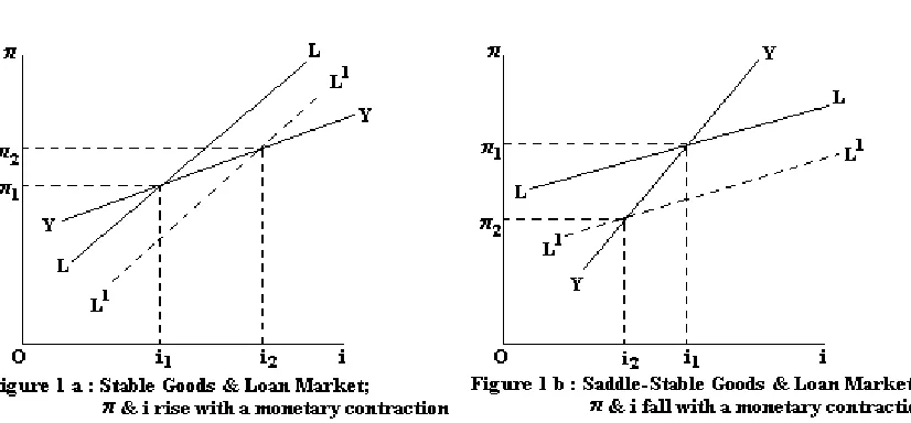
indicates pre (post) -shock interest and inflation rates. Considering the goods and loan

market together we get the structuralist result that a fall in money supply will raise

inflation and interest rates (figure 1a). Under-saddle stability however, both will fall

(figure 1b and appendix). Even so, a fall in money supply reduces inflation in the stable

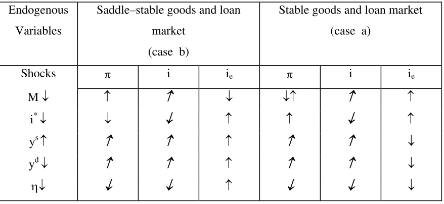
three-market system (figure 2a and Table 2).

Table 2 presents comparative static results for a typical post-stabilisation pattern of

TABLE 2: The Effect of Shocks on Endogenous Variables

Endogenous

Variables

Saddle–stable goods and loan

market

(case b)

Stable goods and loan market

(case a)

Shocks π i ie π i ie

M ↓ ↑ ↑ ↓ ↓↑ ↑ ↑

i* ↓ ↓ ↓ ↑ ↑ ↓ ↑

ys ↑ ↑ ↑ ↑ ↑ ↑ ↓

yd ↓ ↑ ↑ ↑ ↑ ↑ ↓

η↓ ↓ ↓ ↑ ↓ ↓ ↓

Assumptions 1 and 2 and the stability conditions underlie the comparative static results.

Except for i*, the shocks listed in table 2 are typical of a standard reform package. In a

period of structural change, as administrative curbs on asset prices are lifted, the

parameters can change. Two markets interacting together can switch to saddle-stability

and back. But full integration of financial markets will always make the system stable

and reduce sharp fluctuations in asset prices. Only the effects on equity returns and the

effect of money supply on inflation vary under case a and b; the others are invariant, as

the italicised arrows of table 2 indicate. They imply that fluctuations will occur, but in the

net equity indices will fall, interest rates rise, and if the monetary shocks are stronger than

output shocks, inflation may fall under such a structure of shocks.

The new insights in our results are collected in the following propositions:

Proposition 3: A contraction in money supply will raise interest rates but lower inflation,

even in the presence of cost-push from working capital, once equity markets are active.

A monetary contraction can raise interest rates and inflation if

i i e i e

i EE EY EE

EY − > − and under saddle-stability in the goods and loan markets.

Proof: Result R10 (Appendix A.2 (A.2.2)) gives di/dm<0 as

π

πEE EY EE

m will raise i. R8 gives dπ / dm < 0 if EY_ie −EE_ie > EY_i −EE_i. and R9 gives dπ / dm

< 0 under saddle stability (case b).

Q.E.D.

The proposition is illustrated in table 2 and figure 2.

Proposition 4: The affect of stock returns on the goods and stock market excess demands

ensures that a rise (fall) in money supply cannot lead to accelerating (decelerating)

inflation. It follows that a rise in money supply cannot lead to a cumulative rise in

inflation and therefore interest rates.

Proof: EY_ie >EE_ie is assumption 2 which ensuresdi/dm<0or result R10 (Appendix

A.2 (A.2.2)) holds under both case a and b. In the saddle-stable case b a rise in money

supply will cause inflation to fall (R9). But even in the stable case a, if

0 / < −

>

−EE EY EE d dm

EY_{ie ie i i} π , so that inflation will fall with a rise in money

supply (R8). This condition will be met if interest elasticities in the stock and goods

market are high but similar, and the stock market returns have a greater impact on the

goods market excess demands (assumption 2. As stock markets become more important

in the economy EYie will rise. If a rise in money supply does not raise inflationary

expectations it will not raise interest rates through the Fisher effect.

Proposition 5: Where both positive demand and supply shocks occur, the demand shock

must be stronger than the supply shock for inflation and interest rates to fall.

Proof: Result R2(A.2.1 in Appendix A.2), shows that di / dθ < 0 dπ / dθ < 0, whereθis

a positive demand shock. R3 shows that di / dψ > 0 dπ / dψ > 0, whereψis a positive

supply shock. Therefore inflation and interest rates would fall if λ=θ −ψ:or the net

demand shock is positive.

Q.E.D.

Claim 4: As financial markets deepen, a policy configuration that removes impediments

to market integration; adjusts money supply to minimise variation in i; and raises

demand and supply, will deliver the best case scenario of minimum asset price

fluctuations with π and i constant and rising ie.

Proof: Table 2, drawing upon results in Appendix A2, shows that this class of shocks

would lead to the best results. Propositions 1 and 2 demonstrate the tendency for asset

price fluctuations and rising interest sensitivity. Therefore low and stable interest rates

would minimise this volatility, and proposition 4 demonstrates that low i would not result

in inflation.

As asset prices are freed from administrative controls, but other artificial

restrictions on asset market integration continue, the saddle-stable case b is likely to

occur. Without equity markets the structuralist result of a monetary tightening leading to

a rise in inflation does not hold in the saddle-stable case. With equity markets the result

holds in the saddle-stable case, but need not in the other. However, as financial markets

deepen, and equity markets become active, even in this case a, the structuralist result

would be re-established if the impact of stock returns on goods market excess demand is

large. Therefore a monetary policy that is responsive to interest rates is required.

Preliminary tests with daily and monthly asset returns8, interest rates, monetary

aggregates and production and price indices, with Indian data covering the reform period,

provide evidence for the sign restrictions imposed on the partial derivatives and for the

6. Conclusion

Widespread financial deepening, liberalisation and opening make it imperative that

equity and foreign exchange markets are introduced in structuralist theories of asset

markets in developing countries, while retaining features that reflect the structure of such

markets. Another realistic feature of our model is the key role of expectations. Forward

looking inflationary expectations clear the goods market and link it to asset markets.

Assumptions are clearly laid out, and comparative static results derived for alternatives.

The key result that a fall in money supply will raise the rate of inflation now does not

hold under certain conditions, but is re-instated as equity markets become more

important. Moreover, there is a tendency for interest rates to rise and for fluctuations in

asset prices in the short-run. Fuller integration of asset markets moderates these

fluctuations. More active equity markets moderate the impact of a rise on money supply

on inflation. Therefore in transition, a conscious policy stance to keep domestic interest

rates closely linked to foreign, remove artificial barriers to market integration, and

stimulate demand as well as supply, will yield the best results. Although equity returns

can deviate from fundamentals, outcomes can be stable implying that the cause of

financial crises must lie more in high domestic interest rates.

The results are important because of the ambivalent experience many countries

have had with financial reforms, and the fear of crises following the lifting of controls.

But with change in technology controls are difficult to implement. Our results indicate

that partial controls can create more problems, and until viable market institutions

develop the onus is on the monetary authority to ensure liquidity.

The paper can be extended both in theoretical and empirical directions. The sign

restrictions of the excess demand functions can be derived from an explicit maximization

exercise, and the functions can themselves be estimated.

Appendix A

We derive the algebraic expressions for the effects of exogenous shocks on the endogenous variables, by taking total differentials of the excess demand functions.

EE: Excess demand in equity markets

EL: Excess demand in the loan market

EY: Excess demand in the goods market

The three endogenous variables are: ie: the rate of return on equity

i: the loan rate of interest

π: the rate of inflation

The three exogenous shocks we consider are:

η: “news”, a shock impinging on the stock market

m: a rise in the money supply

: ψ θ

λ = − demand shock minus supply shock, or the net demand shock

Two cases affecting the stability of the goods and loan market, for which we work out the results are:

Case a, stability: EY_i > EL_i > EE_i Case b, saddle-stability: EE_i > EL_i > EY_i

EE_π >EL_π >EYπ EE_π >EL_π >EYπ

A.1 The comparative statics of a monetary shock to the goods and loan market

a case b case J EY EL J EL EL EY m i b case a case EL EL EY EY J Since a case b case J EY EL J EL EL EY m m m i i i m i m i 0 0 0 0 0 0 0 0 1 1 1 1 1 < > − = − = δ δ < > − − = < > − = − − − = δ δπ π π π π π R1

Results R1 show that, in case a which is the structuralist –NKE case fall in money supply

will increase the interest rate and inflation.

A.2 Comparative statics: the three markets

0 ) ; , , ( 0 ) ; , , ( 0 ) , , ( /

;

η

π

π

λ

π

i

i

m

i

i

i

i

If all the partial derivatives are taken to be positive, so that the signs are reflected as

pre-fixes: η π π λ π η π π λ π d EE di EE di EE d EE dm EL di EL di EL d EL d EY di EY di EY d EY e ie i m e ie i e ie i − = + − − = + − ± = + −

Writing in matrix form

⎥ ⎥ ⎥ ⎦ ⎤ ⎢ ⎢ ⎢ ⎣ ⎡ − − ± = ⎥ ⎥ ⎥ ⎦ ⎤ ⎢ ⎢ ⎢ ⎣ ⎡ ⎥ ⎥ ⎥ ⎦ ⎤ ⎢ ⎢ ⎢ ⎣ ⎡ − − − ⇒ η λ π η λ π π π d EE dm EL d EL di di d EE EE EE EL EL EL EY EY EY m e ie i ie i ie i (A1)

The Jacobian of partial derivatives is

e e e i i i i i i EE EE EE EL EL EL EY EY EY − − − π π π

The determinant of the Jacobian is:

i i i i i i i i i i EE EE EL EL EY EE EE EL EL EY EE EE EL EL EY J _e e e e e − − − − + + − − = π π π π π

The effect of the exogenous on the endogenous variables can be obtained by applying

Cramer’s rule to equation A1.

A.2.1 Positive demand shock

0 ] [ 0 0 < + − − = − − − − = λ π λ λ J EL EE EE EL EY J EE EE EL EL EY EY EY d

d e e e

e e i i i i i i i i i i R2 0 ] [ 0 0 < − + = − = λ π π λ π π π J EL EE EE EL EY J EE EE EL EL EY EY EY d

di e e e

e e i i i i i R3 J EE EL EE EL EY J EE EE EL EL EY EY EY d

di i i i

i i

e 0 [ ]

0 π π λ π π λ π + − − = − − − − =

λ R4

The sign of die / dλ which depends on the following conditions, gives us results 5 and 6:

R5: Case a (stability) EL_iEE_π >EL_πEE_i

(

)

R6: Case b (saddle-stability) EL_πEE_i >EL_iEE_π

(

)

For a supply shock the signs are reversed since EY_λ >0. Therefore:

R7: dπ/dλ>0, di/dλ >0, and di_e/dλ >0 under saddle-stability but < 0 under stability.

(

)

d i i m i i i i

i i m i i m e e e e e + − = − − − − = π 0 0

R8: dπ/dm>0 under stability (case a) when EE_iEY_ie < EY_iEE_ie . But it can be less than zero if EY_ie−EE_ie > EY_i−EE_i.

R9: dπ / dm < 0 under saddle stability (case b).

J EE EY EE EY EL J EE EE EL EL EL EY EY dm

di ie m ie ie

ie m ie ] [ 0 0 π π π π π − − = − =

R10: di/dm<0 as EY_πEEie < EYi_eEE_π since EYie >EEiefrom assumption 2.

J EE EY EE EY EL J EE EE EL EL EL EY EY dm

di i _{m i i}

m i

i

e 0 [ ]

0 π π π π π + − = − − − − =

R11: di_e/dm>0as EE_πEY_i < EY_πEE_i --case b.

R12: di_e /dm<0as EE_πEY_i > EY_πEE_i --case a.

A.2.3 Shock in world interest rate

An increase in i* will have the same effect as a decrease in m. Therefore the signs of

section A.2.2 are reversed, leading to:

R14: dπ/di*<0,di_e /di*>0 in case a.

A.2.4 Favourable shock to “news” (a fall in international oil prices):

(

)

di ie ie ie

ie ie

(

)

π η η

J EY EL EL EY EE J EE EE EE EL EL EY EY d

d e e e

e e i i i i i i i i i i J EL EY EL EY EE J EE EE EE EL EL EY EY d

di i i i

i i

e [ ]

0 0 π π η η π π π + − − = − − − − = η R15: 0 /dη>

die under case a

0 /dη<

di_e under case b

References

Barro, Robert 1972, A Theory of Monopolistic Price Adjustment, Review of Economic

Studies, 39 (1), Jan., pp.17-26.

Blanchard, O. J. and S. Fischer, 1989, Lectures on Macroeconomics, Cambridge MA:

MIT Press.

Goyal, A. (1999) Developing Economy Macroeconomics: Fresh Perspectives, Allied Publishers, New Delhi.

Goyal, A. (1997) `Sticky Relative Prices, Dynamics and the Closure Debate', Journal of

Post Keynesian Economics, 19,2, 195-222.

Goyal, A. (1995) `The Simple Analytics of Supply, Demand and Structural Adjustment',

Indian Economic Review, 30,2, 37-56.

Goyal, A. (1994) `Growth Dynamics in a General Equilibrium Macroeconomic Model for

India', Journal of Policy Modeling, 16,3, pp. 265-290.

Rotemberg, J.J. and G. Saloner, 1986, A Supergame-theoretic Model of Price Wars

During Booms, American Economic Review 76, 2, 390-407.

Shiller, R., 1981, `Do Stock Prices Move Too Much to Be Justified by Subsequent

Changes in Dividends?’ American Economic Review 71, 3, 421-436.

Shleifer, A. and L.H. Summers, 1990, `The Noise Trader Approach to Finance,' Journal of

Economic Perspectives, 4, 19-33.

Taylor, L., Structuralist Macroeconomics, New York: Basic Books Incorporated, 1983.

Tobin, J. (1982), “Money and Finance in the Macroeconomic Process: Nobel Lecture”, Journal of Money Credit and Banking, 14, 2, 171-202.

Wijnbergen, Van, S., 1983a, Credit Policy Inflation and Growth in a Financially

Repressed Economy, Journal of Development Economics, 13, August, (1-2), pp. 45-66.

Wijnbergen, Van, S., 1983b, Interest Rate Management in LDCs, Journal of Monetary

Economics, 12, September, (3), pp.433-452.

Endnotes

1

There is much commentary in the literature on this result, but the seminal papers were

Taylor 1983, Wijnbergen Van 1983a, b.

2

3_{Walras law imposes the consistency of meeting the budget constraint on schedules of}

supply and demand. For the household portfolio decision, for example, this will imply that the partial derivatives with respect to any interest rate must add up to the partial derivative of wealth demand, with respect to the same variable. Gross substitutability is a stronger assumption and implies that a rise in any interest rate raises the demand for the asset whose yield has increased, without spillover into the other assets. The demand for any asset is positive with respect to own yield but non-positive with respect to other yields. Portfolio theory does not require such a strong assumption (see Tobin 1982). Assets with a strong covariance of yields could be complements. Moreover income effects following the rise in expected yield of any asset can dominate substitution effects. Our assumption 1 imposes Walras law but not gross substitutability of aggregate excess demands.

4_{The assumption is validated by the experience of the nineties in India where} π

z-π was

negative, but gold demand increased steeply inspite of the fall in prices.

5_{India in the nineties provides an interesting illustration of this. While the growth in}

Reserve Bank (RBI) credit to the government was 20.58 in 1990-91 it varied between

only 0.86 and 5.82 over 1991-1995. These were the years when foreign exchange

reserves were built up. RBI credit to the government fell steadily from about 15-16 per

cent of the GDP over 1988-1992 to 10 per cent in 1996-97. The influx of foreign capital

started in 1993.

6_{Stable dynamic adjustment in spite of high induced demand response to exogenous}

shocks is made possible by pricing rules that maximize profits for risk averse firms. Switches between high and low growth equilibria result that are used to understand developing economy macroeconomic outcomes in Goyal 1999. Other relevant articles are Goyal 1994, 1995, 1997. The first applies the analysis to examine agriculture-industry interactions, the second derives aggregate demand and supply curves from it and the third

brings out the implications for closure rules in a general equilibrium model.

7

Noise traders are defined to work with a less than infinite time horizon and to be risk-averse. It has been proved (Shleifer and Summers 1990), that for such traders strategies like "jumping on a bandwagon" or "following a trend" or "stop loss" make profits on average. They would then buy assets when their prices are high, and increase price volatility rather than decrease it. The received wisdom earlier had been that those who buy when high must loose money on average, and would therefore be eliminated. In other words, speculation would help in the revelation of fundamental values. These theories have been validated by much empirical work, starting with Shiller (1981), who showed that volatility in stock prices exceeds that justified by movements in fundamentals.

8_{We first compute simple correlation coefficients between daily asset returns. The data}