Prototype Specification for a Real Computable General Equilibrium Model

Munich Personal RePEc Archive

Prototype Specification for a Real

Computable General Equilibrium Model

Roland-Holst, David and Mensbrugghe, Dominique van der

and Tarp, Finn and Rand, John and Barslund, Mikkel

CIEM

October 2002

Prototype Specification for a Real Computable General Equilibrium Model

David Roland-Holst Dominique van der Mensbrugghe

Finn Tarp John Rand Mikkel Barslund

Table of Contents

INTRODUCTION ... 1

MODEL EQUATIONS ... 2

PRODUCTION ... 2

Top-level nest and producer price ... 2

Second-level production nests ... 3

Third-level production nest ... 4

Fourth-level production nest ... 4

Demand for labor by sector and skill ... 5

Demand for capital and land across types ... 5

Commodity aggregation ... 6

INCOME DISTRIBUTION ... 7

Factor income ... 7

Distribution of profits ... 7

Corporate income ... 8

Household income ... 8

DOMESTIC FINAL DEMAND ... 9

Household expenditures ... 9

Other domestic demand accounts ... 10

TRADE EQUATIONS ... 10

Top-level Armington nest ... 11

Second-level Armington nest ... 11

Top-level CET nest ... 12

Second-level CET nest ... 13

Export demand ... 13

DOMESTIC TRADE AND TRANSPORTATION MARGINS ... 14

GOODS MARKET EQUILIBRIUM ... 14

MACRO CLOSURE ... 15

Government accounts ... 15

Investment and macro closure ... 16

FACTOR MARKET EQUILIBRIUM ... 17

Labor markets ... 17

Capital market ... 18

Land market ... 19

Natural resource market ... 20

MACROECONOMIC IDENTITIES ... 20

GROWTH EQUATIONS ... 21

Model equations ... 21

Equations external to the model ... 21

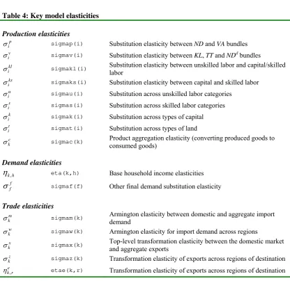
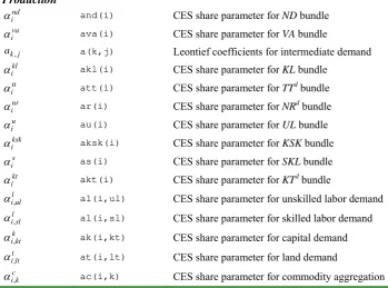
MODEL VARIABLES AND PARAMETERS ... 25

VARIABLE COUNT ... 33

ANNEX 1: LABOR MARKET SEGMENTATION ... 35

Introduction

This document presents a prototype specification for a real computable general equilibrium (CGE) model.1 The prototype has some key features for assessing structural and poverty impacts:

• Labor markets disaggregated by skill level

• Land and capital markets disaggregated by type of capital/land

• A production structure which differentiates the substitutability of unskilled labor on the one hand, and skilled labor and capital on the other hand

• Differentiation of production of like-goods (e.g. small- and large-scale farms, or public versus private production)

• Detailed income distribution

• Intra-household transfers (e.g. urban to rural), transfers from government, and remittances

• Multiple households

• A tiered structure of trade (differentiating across various trading partners)

• Possibility of influencing export prices

• Internal domestic trade and transport margins

• Various potential factor mobility assumptions

• And simple recursive dynamics.

The model has been adapted to help analyze poverty and trade linkages within the context of the inter-agency task force known as the Integrated Framework (IF), and has also been expanded and articulated for a model of China.

The rest of the document proceeds to describe all of the model details using the standard circular flow description of the economy. It starts with production (P), income distribution (Y), demand (D), trade (T), domestic trade and transport margins (M), goods market equilibrium (E), macro closure (C), factor market equilibrium (F), macroeconomic identities (I), and growth (G).

Table 1 describes the indices used in the equations. Note that the model differentiates between production activities, denoted by the index i, and commodities, denoted by the index k. In many models, the two will overlap exactly. However, this differentiation allows for the same commodity to be produced by one or more sectors, and to differentiate these commodities by source of production. For example, it could be used in a model of economies in transition where commodities produced by the public sector have a different cost structure than commodities produced by the private sector, and the commodities themselves could be differentiated by consumers.2 Another example, could be small- versus large-scale agricultural producers.

1 _{Background information on CGE modeling can be found in Derviş et al (1982), Shoven and Whalley (1984 and}

1992), Francois and Reinert (1997) and Hertel (1997).

2 _{The model allows for perfect substitution, in which case consumers are indifferent regarding who produces the}

[image:5.595.117.477.120.331.2]

Table 1: Indices used in the model

i Production activities k Commodities l Labor skills ul Unskilled labor sl Skilled labora kt Capital types lt Land types e Corporations h Households

f Final demand accountsb

m Trade and transport margin accountsc r Trading partners

Notes: a. The unskilled and skilled labor indices, ul and sl, are subsets of l, and their union composes the set indexed by l.

b. The standard final demand accounts are ‘Gov’ for government current expenditures, ‘ZIp’ for private investment, ‘ZIg’ for public investment, ‘TMG’ for international export of trade and transport services, and ‘DST’ for changes in stocks.

c. The standard trade and transport margin accounts are ‘D’ for domestic goods, ‘M’ for imported goods, and ‘X’ for exported goods.

Model Equations

Production

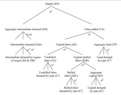
Production, like in most CGE models, relies on the substitution relations across factors of production and intermediate goods. The simplest production structure has a single constant-elasticity-of-substitution (CES) relation between capital and labor, with intermediate goods being used in fixed proportion to output. In the production structure described below, there are multiple types of capital, land and labor, and they are combined in a nested-CES structure intended to represent the various substitution possibilities across these different factors of production. Typically, intermediate goods will enter in fixed proportion to output, though at the aggregate level, the model allows for a degree of substitutability between aggregate intermediate demand and value added.3 The decomposition of value added has several components (see

figure 1 for a representation of the multiple nests). First, land is assumed to be a substitute for an aggregate capital labor bundle.4 The latter is then decomposed into unskilled labor on the one hand, and skilled labor cum capital on the other hand. This conforms to recent observations suggesting that capital and skilled labor are complements, which can substitute for unskilled labor. The four aggregate factors— unskilled and skilled labor, land and capital, are decomposed by type in a final CES nest.

Top-level nest and producer price

The top-level nest has output, XP, produced as a combination of value added, VA, and an aggregate demand for goods and non-factor services, ND. In most cases, the substitution elasticity will be assumed to be zero, in which case the top-level CES nest is a fixed-coefficient Leontief production function. Equations (P-1) and (P-2) represent the optimal demand conditions for the generic CES production function, where PND is the price of the ND bundle, PVA is the aggregate price of value added, PX is the unit cost of production, and σp is the substitution elasticity. If the latter is zero, both ND and VA are used

3 _{Deviations from this structure might include isolating some key inputs, for example energy, or agricultural}

chemicals in the case of crops, and feed in the case of livestock.

4 _{In some sectors the model also allows for a sector-specific factor of production, for example, coal mining and}

in fixed proportions to output, irrespective of relative prices. Equation (P-3) represents the unit cost function, PX. It is derived from the CES dual price formula. The model assumes constant-returns-to-scale and perfect competition in all sectors. Hence, the producer price, PP, is equal to the unit cost, adjusted for a producer tax/subsidy, τp, equation (P-4).

i i i nd i

i XP

PND PX ND

p i

σ

α _⎟⎟

⎠ ⎞ ⎜⎜ ⎝ ⎛

= (P-1)

i i i va i

i XP

PVA PX VA

p i

σ

α _⎟⎟

⎠ ⎞ ⎜⎜ ⎝ ⎛

= (P-2)

) 1 /( 1 1 1

p i p i p

i

i va i i nd i

i PND PVA

PX

σ σ

σ _α

α − − −

⎥⎦ ⎤ ⎢⎣

⎡ ₊

= (P-3)

(

)

i

p i

i PX

PP=1+τ (P-4)

Second-level production nests

The second-level nest has two branches. The first decomposes aggregate intermediate demand, ND, into sectoral demand for goods and services, XAp. The model explicitly assumes a Leontief structure. Thus equation (P-5) describes the demand for good k by sector j, where the coefficient a represents the proportion between XAp and ND. The price of the ND bundle, PND, is the weighted average of the price of goods and services, PA, using the technology coefficients as weights, equation (P-6). The so-called Armington price is multiplied by a sector and commodity specific indirect tax, τcp.

j j k j

k a ND

XAp , = , (P-5)

(

)

∑

+

=

k

k cp

j k j k

j a PA

PND , 1 τ _, (P-6)

The second branch decomposes the aggregate value added bundle, VA, into three components: aggregate demand for capital and labor, KL, aggregate land demand, TTd, and a sector-specific resource, NR,5 see equations (P-7) through (P-9). The relevant component prices are PKL, PTT and PR, respectively, and the substitution elasticity is given by σv. Equation (P-9) allows for the possibility of factor productivity changes as represented by the λ parameter. The price of value added, PVA, is the CES aggregation of the three component prices, as defined by equation (P-10).

i i i kl i i VA PKL PVA KL v i σ α _⎟⎟ ⎠ ⎞ ⎜⎜ ⎝ ⎛

= (P-7)

i i i tt i d i VA PTT PVA TT v i σ α _⎟⎟ ⎠ ⎞ ⎜⎜ ⎝ ⎛

= (P-8)

( )

i

i i nr i nr i d i VA PR PVA NR v i v i σ σ λ α _⎟⎟ ⎠ ⎞ ⎜⎜ ⎝ ⎛

= −1 (P-9)

) 1 /( 1 1 1 1 v i v i v i v i nr i i nr i i tt i i kl i i PR PTT PKL PVA σ σ σ σ λ α α α − − − − ⎥ ⎥ ⎥ ⎦ ⎤ ⎢ ⎢ ⎢ ⎣ ⎡ ⎟ ⎟ ⎠ ⎞ ⎜ ⎜ ⎝ ⎛ + +

= (P-10)

Third-level production nest

The third-level nest decomposes the aggregate capital-labor bundle, KL, into two components. The first is the aggregate demand for unskilled labor, UL, with an associated price of PUL. The second is a bundle composed of skilled labor and capital, KSK, with a price of PKSK. Equations (P-11) and (P-12) reflect the standard CES optimality conditions for the demand for these two components, with a substitution elasticity given by σkl. The price of capital-labor bundle, PKL, is defined in equation (P-13).

i i i u i i KL PUL PKL UL kl i σ α _⎟⎟ ⎠ ⎞ ⎜⎜ ⎝ ⎛

= (P-11)

i i i ksk i i KL PKSK PKL KSK kl i σ α _⎟⎟ ⎠ ⎞ ⎜⎜ ⎝ ⎛

= (P-12)

) 1 /( 1 1 1 kl i kl i kl i i ksk i i u i

i PUL PKSK

PKL

σ σ

σ _α

α − − −

⎥⎦ ⎤ ⎢⎣

⎡ ₊

= (P-13)

Fourth-level production nest

i i i s i i KSK PSKL PKSK SKL ks i σ α _⎟⎟ ⎠ ⎞ ⎜⎜ ⎝ ⎛

= (P-14)

i i i kt i d i KSK PKT PKSK KT ks i σ α _⎟⎟ ⎠ ⎞ ⎜⎜ ⎝ ⎛

= (P-15)

) 1 /( 1 1 1 ks i ks i ks i i kt i i s i

i PSKL PKT

PKSK

σ σ

σ _α

α − − −

⎥⎦ ⎤ ⎢⎣

⎡ ₊

= (P-16)

Demand for labor by sector and skill

Equations (P-17) and (P-18) decompose the demands for aggregate unskilled and skilled labor, respectively, across their different components. The variable Ld represents labor demand in sector i for labor of skill level l. The relevant wage is given by W which is allowed to be both sector and skill-specific. The respective cross-skill substitution elasticities are σu and σs. Both equations (P-17) and (P-18) incorporate sector and skill specific labor productivity, represented by the variable λl. The aggregate unskilled and skilled price indices are determined in equations (P-19) and (P-20), respectively PUL and

PSKL.

( )

i

ul i i l ul i l ul i d ul i UL W PUL L u i u i σ σ λ

α _⎟⎟

⎠ ⎞ ⎜ ⎜ ⎝ ⎛ = − , 1 , ,

, for ul∈{Unskilledlabor} (P-17)

( )

i

sl i i l sl i l sl i d sl i SKL W PSKL L s i s i σ σ λ

α _⎟⎟

⎠ ⎞ ⎜ ⎜ ⎝ ⎛ = − , 1 , ,

, for sl∈{Skilledlabor} (P-18)

) 1 /( 1 } labor Unskilled { 1 , , , u i u i ul l ul i ul i l ul i i W PUL σ σ λ α − ∈ − ⎥ ⎥ ⎥ ⎦ ⎤ ⎢ ⎢ ⎢ ⎣ ⎡ ⎟ ⎟ ⎠ ⎞ ⎜ ⎜ ⎝ ⎛

=

∑

(P-19)

) 1 /( 1 } labor Skilled { 1 , , , s i s i sl l sl i sl i l sl i i W PSKL σ σ λ α − ∈ − ⎥ ⎥ ⎥ ⎦ ⎤ ⎢ ⎢ ⎢ ⎣ ⎡ ⎟ ⎟ ⎠ ⎞ ⎜ ⎜ ⎝ ⎛

=

∑

(P-20)

Demand for capital and land across types

( )

d i kt i i k kt i k kt i d kt i KT R PKT K k i k i σ σ λ

α _⎟⎟

⎠ ⎞ ⎜ ⎜ ⎝ ⎛ = − , 1 , ,

, (P-21)

) 1 /( 1 1 , , , k i k i kt k kt i kt i k kt i i R PKT σ σ λ α − − ⎥ ⎥ ⎥ ⎦ ⎤ ⎢ ⎢ ⎢ ⎣ ⎡ ⎟ ⎟ ⎠ ⎞ ⎜ ⎜ ⎝ ⎛

=

∑

(P-22)

( )

d

i lt i i t lt i t lt i d lt i TT PT PTT T t i t i σ σ λ

α _⎟⎟

⎠ ⎞ ⎜ ⎜ ⎝ ⎛ = − , 1 , ,

, (P-23)

) 1 /( 1 1 , , , t i t i lt t lt i lt i t lt i i PT PTT σ σ λ α − − ⎥ ⎥ ⎥ ⎦ ⎤ ⎢ ⎢ ⎢ ⎣ ⎡ ⎟ ⎟ ⎠ ⎞ ⎜ ⎜ ⎝ ⎛

=

∑

(P-24)

Commodity aggregation

Each activity produces a single commodity, XP, indexed by i. Consumption goods, indexed by k, are a combination of one or more produced goods. Aggregate domestic supply of good k, X, is a CES combination of one or more produced goods i. In many cases, the CES aggregate is of a single commodity, i.e. there is a one-to-one mapping between a consumed good and its relevant production. There are cases, however, where it is useful to have consumed goods be an aggregation of produced goods, for example when combining similar goods with different production characteristics (e.g. public versus private, commercial versus small-scale, etc.) Equation (P-25) represents the optimality condition of the aggregation of produced goods into commodities. The producer price is PP, and the price of the aggregate supply is P. The degree of substitutability across produced commodities is σc. Equation (P-26) determines the aggregate supply price, P. The model allows for perfect substitutability, in which case the law of one price holds and the produced commodities are simply aggregated to form aggregate output.6

⎪ ⎩ ⎪ ⎨ ⎧ ∞ = = ∞ ≠ ⎟⎟ ⎠ ⎞ ⎜⎜ ⎝ ⎛ = c k k i c k k i k c k i i P PP X PP P XP c k σ σ α σ if if

, _(P-25)

⎪ ⎪ ⎩ ⎪ ⎪ ⎨ ⎧ ∞ = = ∞ ≠ ⎥ ⎥ ⎦ ⎤ ⎢ ⎢ ⎣ ⎡ =

∑

∑

∈ − ∈ − c k K i i k c k K i i c k i k XP X PP P c k c k σ σ α σ σ if if ) 1 /( 1 1 , (P-26)

6 _{Electricity is a good example of a homogeneous output but which could be produced by different production}

Income distribution

The prototype model has a rich menu of income distribution channels—factor income and intra-household, government and foreign transfers (i.e. remittances). The prototype also includes corporations used as a pass-through account for channeling operating surplus.

Factor income

There are four broad factors—a sector specific resource, land, labor and capital—the latter three which can be sub-divided into various types. Equations (Y-1) through (Y-4) determine aggregate net-income from labor, LY, capital, KY, land, TY, each indexed by their respective sub-types, and the sector specific factor, RY. These are net incomes because the model incorporates factor taxes designated by τfl, τfk, τft and

τfr

respectively.7

∑

₊

=

i fl

l i

d l i l i l

L W LY

, , ,

1 τ (Y-1)

∑

₊

=

i

fk kt i

d kt i kt i kt

K R KY

, , ,

1 τ (Y-2)

∑

₊

=

i

ft lt i

d lt i lt i lt

T PT TY

, , ,

1 τ (Y-3)

∑

₊

=

i

fr i

d i iNR PR RY

τ

1 (Y-4)

Distribution of profits

All of labor, land and sector-specific factor income is allocated directly to households.8 Profits (aggregated with income from the sector-specific resouce), on the other hand, are distributed to three broad accounts, enterprises, households, and the rest of the world (ROW). Equation (Y-5) determines the level of profits distributed to enterprises, TRE. Equation (Y-6) represents the level of profits distributed directly to households, TRH. And, equation (Y-7) determines the level of factor income distributed abroad,

TRW. Note that the three share parameters, ϕE, ϕH, and ϕW sum to unity.

kt E

kt k E

kt

k KY

TR _, =ϕ _, (Y-5)

kt H

kt k H

kt

k KY

TR _, =ϕ _, (Y-6)

kt W

kt k W

kt

k KY

TR _, =ϕ _, (Y-7)

7 _{The factor taxes are type- and sector-specific. Note as well that the relevant factor prices represent the perceived}

cost to employers, not the perceived remuneration of workers.

8 _{Depending on the structure of the final SAM, land and or income from the sector-specific resource may also}

Corporate income

Corporate income, TRE, is split into four accounts. First, the government receives its share through the corporate income tax, κc. The residual is split into three: retained earnings, and income distributed to households and the rest of the world. Equation (Y-8) determines corporate income of enterprise e, CY. It is the sum, over possible capital types, of shares of distributed profits (to corporations).9 Equation (Y-9) determines retained earnings, i.e. corporate savings, Sc, where the rate of retained earnings is given by sc. Equations (Y-10) and (Y-11) determine the overall transfers to households and to ROW. Note that the two share parameters, ϕH and ϕW, and the retained earnings rate, sc, sum to unity.

∑

=

kt

E kt k e

e kt

e TR

CY ϕ _{, ,} (Y-8)

(

)

e

c e c e c

e s CY

S = 1−κ (Y-9)

( )

e

c e H

e c H

e

c CY

TR_, =ϕ_, 1−κ (Y-10)

( )

e

c e W

e c W

e

c CY

TR_, =ϕ_, 1−κ (Y-11)

Household income

Aggregate household income, YH, is composed of eight elements: labor, land and sector-specific factor remuneration, distributed capital income and corporate profits, transfers from government and households, and foreign remittances, equation (Y-12).10 Government transfers, in the standard closure, are fixed in real terms and are multiplied by an appropriate price index to preserve model homogeneity. Remittances, are fixed in international currency terms, and are multiplied by the exchange rate, ER, to convert them into local currency terms.11

9 _{The share parameters, ϕ}e

, sum to unity.

10 _{All share parameters within the summation signs sum to unity.}

43 42 1 43 42 1 4 43 4 42 1 4 4 3 4 4 2 1 43 42 1 43 42 1 4 4 3 4 4 2 1 43 42 1 s remittance Foreign , s transfer household -Intra ' ' , government from Transfers , Enterprise , , factor specific -Sector , Land , Capital , , Labor , .

. _Wh _h

h h h h H h g e H e c h h e h h nr lt lt h h lt kt H kt k h h kt l l h h l h TR ER TR TR PLEV TR RY TY TR LY YH + + + + + + + =

∑

∑

∑

∑

∑

ϕ ϕ ϕ ϕ ϕ (Y-12)

(

)

H

h h h h h

h YH TR

YD =1−λκ − (Y-13)

(

)

h

h h h H h h H h YH

TR =ϕ , 1−λκ (Y-14)

H h h h h h h h TR

TR ,'=ϕ , ' ' (Y-15)

H h W h W h TR

TR =ϕ (Y-16)

Disposable income, YD, is equal to after-tax income, less household transfers, equation (Y-13), where the household tax rate is κh. It is multiplied by an adjustment factor, λh, which is used for model closure. In the standard closure, government savings (or deficit), is held fixed, and the household tax schedule adjusts (uniformly) to achieve the given government fiscal balance. In other words, under this closure rule, the relative tax rates across households remain constant.12 Aggregate household transfers, TRH, is a share of after tax income, equation (Y-14). This is transferred to individual households and abroad, respectively

TRh and TRW, using constant share equations, (Y-15) and (Y-16).

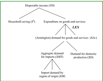
Domestic final demand

Domestic final demand is composed of two broad agents—households and other domestic final demand. The model incorporates multiple households. Household demand has a uniform specification, however, with household-specific expenditure parameters. The other domestic final demand categories, in the standard model, include government current expenditures, Gov, private and public investment expenditures, ZIp and ZIg, exports of international trade and transport services, TMG, and changes in stocks, DST. The other domestic final demand categories, indexed by f, are also assumed to have a uniform expenditure function, but with agent-specific expenditure parameters. Demand at the top-level, reflects demand for the Armington good. The latter are added up across all activities in the economy and split into domestic and import components at the national level.13

Household expenditures

Households have a tiered demand structure, see figure 2. At the top-level, households save a constant share of disposable income, with the savings rate given by sh. At the next level, residual income is allocated across goods and services, XAc, using the linear expenditure system (LES).14 Equation (D-1) represents the LES demand function. Household consumption is the sum of two components. The first, θ,

12 _{An alternative would be to use an additive factor, which would adjust the average tax rates, not the marginal tax}

rates.

13 _{There are few SAMs, which would allow for agent-specific Armington behavior.}

14 _{This class of models often uses the so-called extended linear expenditure system, which integrates household}

is referred to as the subsistence minimum, or floor consumption.15 The second is a share of supernumerary income, or discretionary income. Supernumerary income is equal to residual disposable income, subtracting savings and aggregate expenditures on the subsistence minima from disposable income. The next level, undertaken at the national level, is the decomposition of Armington demand, XAc, into its domestic and import components, see below. Equation (D-2) determines household saving, Sh, by residual. The consumer price index, CPI, is defined in equation (D-3). Note that the consumer price is equal to the economy-wide Armington price, PA, multiplied by a household and commodity specific ad valorem tax, τcc.

⎟ ⎟ ⎠ ⎞ ⎜ ⎜ ⎝ ⎛ + − − + + =

∑

' ,' ' ,' , , ,

, (1 ) (1 )

) 1

( _k k h kh

cc h k h h h k cc h k h k h k h h

k s YD PA Pop

PA Pop

XAc τ θ

τ μ

θ (D-1)

∑

+ − = k h k k cc h k h h

h YD PA XAc

S (1 τ _, ) _, (D-2)

∑

∑

+ + = k h k k cc h k k h k k cc h k h XAc PA XAc PA CPI 0 , , 0 , 0 , , 0 , , , ) 1 ( ) 1 ( τ τ (D-3)

Other domestic demand accounts

The other domestic final demand accounts all use a CES expenditure function (with the option of having fixed volume or value expenditure shares with an elasticity of 0 or 1, respectively). Equation (D-4) determines the expenditure share on goods and services, XAf. Equation (D-5) defines the expenditure price index, PF. And equation (D-6) defines the value of expenditures, YF. Model closure is discussed below. f k cf f k f f f k f k XF PA PF XAf f f σ τ

α _⎟⎟

⎠ ⎞ ⎜ ⎜ ⎝ ⎛ + = ) 1 ( _, ,

, (D-4)

(

)

1/(1 ) 1

,

, (1 )

f f f f k k cf f k f f k f PA PF σ σ τ α − − ⎥ ⎥ ⎦ ⎤ ⎢ ⎢ ⎣ ⎡ +

=

∑

(D-5)

f f

f PF XF

YF = (D-6)

Trade equations

This section discusses the modeling of trade. There are three sections—import demand, and export supply and demand. The first two use a tiered structure. Import demand is decomposed in two steps. The top tier disaggregates aggregate Armington demand into two components—demand for the domestically produced good and aggregate import demand. At the second tier, the aggregate import demand is

allocated across trading partners. Both of these tiers assume that goods indexed by k are differentiated by region of origin, i.e. the so-called Armington assumption.16 A CES specification is used to model the degree of substitutability across regions of origin. The level of the elasticities will often be determined by the level of aggregation. Finely defined goods, such as wheat, would typically have a higher elasticity than more broadly defined goods, such as clothing. At the same time, non-price barriers may also inhibit the degree of substitutability, for example prohibitive transport barriers (inexistent or few transmission lines for electricity), or product and safety standards. Export supply is similarly modeled using a two-tiered constant-elasticity-of-transformation specification. This permits imperfect supply responses to changes in relative prices. Finally, the small-country assumption is relaxed for exports with the incorporation of export demand functions.

Top-level Armington nest

National demand for the Armington good, XA, is the sum of Armington demand over all domestic agents: intermediate demand, household and other domestic final demand, and demand generated by the internal trade and transport sector, XAmg, equation (T-1). Aggregate Armington demand is then allocated between domestic and import goods using a nested CES structure. Equation (T-2) represents demand for the domestically produced good, XDd, where the top-level Armington elasticity is given by σm. Note that the price of the domestic good is equal to the producer price, PD, adjusted by the internal trade and transport margin, τmg. Demand for aggregate imports, XMT, is determined in equation (T-3). The price of aggregate imports is given by PMT.17 The Armington price, PA, is defined in equation (T-4), using the familiar CES dual price aggregation formula.

∑∑

∑

∑

∑

+ + +

=

m k

m k k f

f k h

h k j

j k

k XAp XAc XAf XAmg

XA

'

,' , ,

,

, (T-1)

k k mg

D k

k d

k d

k XA

PD PA XD

m k

σ

τ

α _⎟⎟

⎠ ⎞ ⎜

⎜ ⎝ ⎛

+ =

) 1

( _, (T-2)

k k k m k

k XA

PMT PA XMT

m k

σ

α _⎟⎟

⎠ ⎞ ⎜⎜ ⎝ ⎛

= (T-3)

(

)

1/(1 )

1 1

, )

1 (

m k m k m

k

k m k k

mg D k d k

k PD PMT

PA

σ σ σ

α τ

α

− − −

⎥⎦ ⎤ ⎢⎣

⎡ _{+ +}

= (T-4)

Second-level Armington nest

At the second level, aggregate import demand, XMT, is allocated across trading partners using a CES specification. Equation (T-5) defines the domestic price of imports, PM.18 It is equal to the world price (in international currency), WPM, multiplied by the exchange rate, and adjusted for by the import tariff, τm, i.e. PM represents the port-price of imports, tariff-inclusive. The tariff rate is both sector- and region of origin-specific. The tariff rate is also multiplied by a uniform shifter, χtm, which is normally equal to 1.

16 _{The seminal article on product differentiation in trade is Armington (1969). See also de Melo and Robinson}

(1989).

The shifter can be modified exogenously for specific simulations, for example setting it to 0.5 would cut tariffs by 50 percent across the board, or it can be rendered endogenous, assuming there is an exogenous target to be achieved. For example, to calculate a uniform revenue neutral tariff rate, one could set all tariffs (or positive-rated tariffs) to 0.1 and endogenize the shift parameter, χtm. The exogenous variable is the value of initial tariff revenues (in real terms). If the calculated χtm is 1.5, this indicates that the uniform revenue neutral tariff is 15 percent. Equation (T-6) represents the import of commodity k from region r,

XM, where the inter-regional substitution elasticity is given by σw. The relevant consumer price includes the internal trade and transport margin, τmg. The aggregate price of imports, PMT, is defined in equation (T-7).

) 1

(

. , ,

,

m r k tm r k r

k ERWPM

PM = +χ τ (T-5)

k r

k mg

M k

k w

r k r

k XMT

PM PMT XM

w k

σ

τ

α _⎟⎟

⎠ ⎞ ⎜

⎜ ⎝ ⎛

+ =

, ,

, ,

) 1

( (T-6)

(

)

1/(1 ) 1

, ,

, (1 )

w k w k

r

r k mg

M k w

r k

k PM

PMT

σ σ

τ α

− −

⎥ ⎥ ⎦ ⎤ ⎢

⎢ ⎣ ⎡

+

=

∑

(T-7)

Top-level CET nest

Domestic production is allocated across markets using a nested CET specification. At the top nest, producers allocate production between the domestic market and aggregate exports. At the second nest, aggregate exports are allocated across trading partners. The model allows for perfect transformation, i.e. producers perceive no difference across markets. In this case, the law-of-one-price holds. Equation (T-8) represents the link between the domestic producer price, PE, and the world price, WPE. Export prices are both sector- and region-specific. The FOB price, WPE, includes domestic trade and transport margins,

τmg19

, as well as export taxes/subsidies, τe. Equations (T-9) and (T-10) represent the CET optimality conditions. The first determines the share of domestic supply, X, allocated to the domestic market, XDs. The second determines the supply of aggregate exports, XET. PET represents the price of aggregate export supply. The transformation elasticity is given by σx. The model allows for perfect transformation. In this case, the optimal supply conditions are replaced by the law-of-one price conditions. Equation (T-11) represents the CET aggregation function. In the case of finite transformation, it is replaced with its equivalent, the CET dual price aggregation function. In the case of infinite transformation, the primal aggregation function is used, where the two components are summed together since there is no product differentiation.

19 _{Note that the domestic trade and transport margins are differentiated for three different goods: domestically}

(

)(

)

kr e r k mg X k r

k ERWPE

PE, 1+τ , 1+τ , = . , (T-8)

⎪ ⎪ ⎩ ⎪⎪ ⎨ ⎧ ∞ = = ∞ ≠ ⎟⎟ ⎠ ⎞ ⎜⎜ ⎝ ⎛ = x k k k x k k k k d k s k P PD X P PD XD x k σ σ γ σ if

if _(T-9)

⎪ ⎪ ⎩ ⎪⎪ ⎨ ⎧ ∞ = = ∞ ≠ ⎟⎟ ⎠ ⎞ ⎜⎜ ⎝ ⎛ = x k k k x k k k k e k k P PET X P PET XET x k σ σ γ σ if

if _(T-10)

⎪⎩ ⎪ ⎨ ⎧ ∞ = + = ∞ ≠ ⎥⎦ ⎤ ⎢⎣ ⎡ ₊ = + + + x k k s k k x k k e k k d k k XET XD X PET PD P x k x k x k σ σ γ

γ σ σ σ

if if ) 1 /( 1 1 1 (T-11)

Second-level CET nest

The second-level CET nest allocates aggregate export supply, XET, across the various export markets,

XE. Equation (T-12) represents the optimal allocation decision, where σz is the transformation elasticity. Equation (T-13) represents the CET aggregation function, where again, the CET dual price formula is used to determine the aggregate export price, PET. As above, the model allows the transformation elasticity to be infinite.

⎪ ⎪ ⎩ ⎪⎪ ⎨ ⎧ ∞ = = ∞ ≠ ⎟⎟ ⎠ ⎞ ⎜⎜ ⎝ ⎛ = z k k r k z k k k r k x r k r k PET PE XET PET PE XE z k σ σ γ σ if if , , ,

, _(T-12)

⎪ ⎪ ⎩ ⎪ ⎪ ⎨ ⎧ ∞ = = ∞ ≠ ⎥ ⎥ ⎦ ⎤ ⎢ ⎢ ⎣ ⎡ =

∑

∑

+ + z k r r k k z k r r k x r k k XE XET PE PET z k z k σ σ γ σ σ if if , ) 1 /( 1 1 , , (T-13) Export demand

⎪ ⎪ ⎩ ⎪⎪ ⎨ ⎧

∞ = =

∞ ≠ ⎟

⎟ ⎠ ⎞ ⎜

⎜ ⎝ ⎛ =

e r k r

k r

k

e r k r

k r k e

r k r k

WPE WPE

WPE WPE ED

e r k

, ,

,

, ,

, ,

,

if if

,

η η α

η

(T-14)

Domestic trade and transportation margins

The marketing of each good—domestic, imports, and exports—is associated with a commodity specific trade margin.20 Equations (M-1) through (M-3) define the revenues associated with the domestic trade and transport margins. Domestically produced goods sold domestically generate Y.,mgD . Imported goods

generate Y.,mgM . And exported goods generate mg

X

Y_., . Equation (M-4) defines the volume of margin services. The production of the trade and transport services follows a Leontief technology. Equation (M-5) defines the demand for goods and services. In other words, to deliver commodity k' (in either sector D, M, or X) requires an input from commodity k, the level of which is fixed in proportions to the overall volume of delivering commodity k' in the economy, XTkmg' . Equation (M-6) is the expenditure deflator,

mg k

PT_' , for individual trade margin activities.

d k k mg

D k mg

D

k PD XD

YT_, =τ _, (M-1)

∑

=

r

r k r k mg

M k mg

M

k PM XM

YT, τ , , , (M-2)

∑

=

r

r k r k mg

X k mg

X

k PE XE

YT_, τ _{, , ,} (M-3)

mg m k mg

m k mg

m

k YT PT

XT _, = _, / _, (M-4)

mg m k mg

m k k m k

k XT

XAmg , ,' =α _{, ', ,'} (M-5)

∑

=

k

k mg

m k k mg

m

k PA

PT _,' α _{, ,'} (M-6)

Goods market equilibrium

There are three fundamental commodities in the model—domestic goods sold domestically, imports (by region of origin), and exports (by region of destination). All other goods are bundles (i.e. are defined using an aggregation function) and do not require supply/demand balance. The small-country assumption holds for imports, and therefore any import demand can be met by the rest of the world with no impact on the price of imports. Therefore, there is no explicit supply/demand equation for imports.21 Equation (E-1) represents equilibrium on the domestic goods market, and essentially determines, PD, the producer price of the domestic good. Equation (E-2) defines the equilibrium condition on the export market. With a finite

20 _{The model does not include international trade and transport margins. A change in the latter could be simulated}

by a change in the relevant world price index, WPM or WPE.

export demand elasticity, the equation determines WPE, the world price of exports. With an infinite export demand elasticity, the equation trivially equates export supply to the given export demand.

s k d

k XD

XD = (E-1)

r k r

k XE

ED, = , (E-2)

Macro closure

Macro closure involves determining the exogenous macro elements of the model. The standard closure rules are the following:

• Government fiscal balance is exogenous, achieved with an endogenous direct tax schedule

• Private investment is endogenous and is driven by available savings

• The volume of government current and investment expenditures is exogenous

• The volume of demand for international trade and transport services is exogenous

• The volume of stock changes is exogenous

• The trade balance (i.e. capital flows) is exogenous. The real exchange rate equilibrates the balance of payments.

These are detailed further below.

Government accounts

Equation (C-1) describes nominal tariff revenues, TarY, and equation (C-2) defines real tariff revenues,

∑∑

= k r r k r k m r k tm XM WPM ER

TarY χ τ , , , (C-1)

PLEV TarY

RTarY= / (C-2)

43 42 1 4 43 4 42 1 43 42 1 4 4 3 4 4 2 1 4 4 3 4 4 2 1 4 4 3 4 4 2 1 4 4 4 3 4 4 4 2 1 4 4 4 3 4 4 4 2 1 4 4 4 4 4 4 4 3 4 4 4 4 4 4 4 2 1 4 4 4 4 3 4 4 4 4 2 1 4 4 4 3 4 4 4 2 1 4 4 4 3 4 4 4 2 1 ROW from Transfers tax Income tax Corporate tax Production tax Resource tax Wage , , , , tax Capital , , , , tax Land , , , , revenues x export ta and iff Import tar , , , , demand final other on tax Sales , , demand household on tax Sales , , demand te intermedia on tax Sales , , . 1 1 1 1 ) 1 ( g W h h h h h e e c e i i i p i i fr i d i i fr i l i fl l i d l i l i fl l i kt i fk kt i d kt i kt i fk kt i lt i ft lt i d lt i lt i ft lt i k r r k r k mg X k e r k k f f k k cf f k k h h k k cc h k k j j k k cp j k TR ER YH CY XP PX NR PR L W K R T PT XE PE TarY XAf PA XAc PA XAp PA GY + + + + + + + + + + + + + + + + + =

∑

∑

∑

∑

∑∑

∑∑

∑∑

∑∑

∑∑

∑∑

∑∑

κ λ κ τ τ τ τ τ τ τ τ τ τ τ τ τ τ (C-3) W g h H h g

Gov PLEV TR ERTR

YF

GEXP= +

∑

_, + . (C-4)

GEXP GY

Sg = − (C-5)

PLEV S

RSg= g/ (C-6)

Investment and macro closure

f g

h h h e

c e DST

ZIg

ZIp YF YF S S S ERS

YF + + =

∑

+

∑

+ + . (C-7)

Gov

Gov XF

XF = (C-8)

ZIg

ZIg XF

XF = (C-9)

TMG

TMG XF

XF = (C-10)

DST

DST XF

XF = (C-11)

∑

∑

=

k

k k k

k k

XA PA

XA PA

PLEV

0 , 0 ,

0 ,

(C-12)

0

, ,

, ,

, ,

,

≡

− +

+ −

−

+ + +

+ =

∑

∑

∑

∑∑

∑

∑∑

W g h

W h e

W e c kt

W kt k

r k

r k r k

f g W h

h h W TMG

r k

r k r k

TR ER

TR TR

TR

XM WPM

S TR TR YF

XE WPE BoP

(C-13)

Factor market equilibrium

The following sections describe the standard factor market equilibrium conditions.22

Labor markets

Labor markets are assumed to clear. Equation (F-1) describes the upward sloping labor supply curve, including the two polar cases of a vertical supply curve (ωl = 0) and a horizontal supply curve, i.e. an infinite elasticity, in which case the real wage is fixed. Equation (F-2) sets aggregate demand, by skill-level, equal to aggregate supply, Ls. This equation determines the equilibrium wage, We.23 Equation (F-3) equates sectoral wages to the equilibrium wage, but allows for a fixed sector-specific relative wage factor,

φl .24

22 _{More detailed analysis may require more market segmentation, e.g. rural versus urban labor markets, though}

some of this segmentation can be picked up by the data itself.

23 _{Market structure can emulate perfect market segmentation by an appropriate definition of labor skills. For}

example, unskilled rural labor can assume to be only employed in rural sectors, whereas unskilled urban labor is only employed in urban sectors. Perfect market segmentation, as modeled here, does not allow for migration.

24 _{Quite a few alternatives could be used to endogenize relative sector-specific wages, for example union wage}

⎪ ⎪ ⎩ ⎪⎪ ⎨ ⎧

∞ = =

∞ ≠ ⎟

⎟ ⎠ ⎞ ⎜ ⎜ ⎝ ⎛ =

l e

l e

l

l e

l ls l s l

W PLEV W

PLEV W L

l

ω ω α

ω

if .

if

0 ,

(F-1)

∑

=

i d

l i s

l L

L . (F-2)

e l l

l i l

i W

W_, =φ_, (F-3)

Capital market

Equilibrium on the capital market allows for both limiting cases—perfect capital mobility and perfect capital immobility, or any intermediate case. Aggregate capital, Ks, is allocated across sectors and type according to a nested CET system. At the top-level, the aggregate investor allocates capital across types, according to relative rates of return. Equation (F-4) determines the optimal supply decision, where TKs is the supply of capital of type kt, with an average return of PTK. PK is the aggregate rate-of-return to capital. If the supply elasticity is infinite, the law-of-one-price holds. Equation (F-5) represents the top-level aggregation function, replaced by the CET dual price function in the case of a finite transformation elasticity. Perfect capital mobility is represented by setting ωkt to infinity. Perfect immobility is modeled by setting the transformation elasticity to 0.

⎪ ⎩ ⎪ ⎨ ⎧

∞ = =

∞ ≠ ⎟

⎠ ⎞ ⎜ ⎝ ⎛ =

kt kt

kt s

kt tks kt s kt

PK PTK

K PK PTK TK

kt

ω ω

γ ω

if

if _(F-4)

⎪ ⎪ ⎩ ⎪ ⎪ ⎨ ⎧

∞ = =

∞ ≠ ⎥

⎥ ⎦ ⎤ ⎢

⎢ ⎣ ⎡ =

∑

∑

+ +

kt

kt s kt s

kt

kt

kt tks kt

TK K

PTK PK

kt kt

ω ω γ

ω ω

if if

) 1 /( 1 1

(F-5)

At the second level, capital by type, TKs, is allocated across sectors using another CET function. Equation (F-6) determines the optimal allocation of capital of type kt to sector i, Ks, where the transformation elasticity is ωk. Equation (F-7) represents the CET aggregation function. The equilibrium return to capital,

R, is determined by equation capital supply to demand, equation (F-8).25

25 _{If the transformation elasticity is infinite, equation (F-6) determines the sector- and type-specific rate of return}

⎪ ⎪ ⎩ ⎪⎪ ⎨ ⎧ ∞ = = ∞ ≠ ⎟⎟ ⎠ ⎞ ⎜⎜ ⎝ ⎛ = k kt kt i k s kt kt kt i k kt i s kt i PTK R TK PTK R K k ω ω γ ω if if , , ,

, _(F-6)

⎪ ⎪ ⎩ ⎪ ⎪ ⎨ ⎧ ∞ = = ∞ ≠ ⎥ ⎥ ⎦ ⎤ ⎢ ⎢ ⎣ ⎡ =

∑

∑

+ + k i s kt i kt k i kt i k kt i kt K TK R PTK k k ω ω γ ω ω if if , ) 1 /( 1 1 , , (F-7) d kt i s kt i K

K, = , (F-8)

Land market

Land market equilibrium is specified in an analogous way to the capital market with a tiered CET supply system. The first tier allocates total land across types. This could have a zero transformation elasticity if for example land used for rice production could not be used to produce other commodities. Their respective prices are PLAND and PTTs.

⎪ ⎪ ⎩ ⎪⎪ ⎨ ⎧ ∞ = = ∞ ≠ ⎟ ⎟ ⎠ ⎞ ⎜ ⎜ ⎝ ⎛ = tl s lt tl s lt tts lt s lt PLAND PTT LAND PLAND PTT TT tl ω ω γ ω if

if _(F-9)

( )

⎪ ⎪ ⎩ ⎪ ⎪ ⎨ ⎧ ∞ = = ∞ ≠ ⎥ ⎥ ⎦ ⎤ ⎢ ⎢ ⎣ ⎡ =

∑

∑

+ + tl lt s lt tl lt s lt tts lt TT LAND PTT PLAND tl tl ω ω γ ω ω if if ) 1 /( 1 1 (F-10)

Equations (F-11) and (F-12) determine the optimality conditions at the second and final tier, determining land supply (by type and) by sector of use. Land market equilibrium is represented by equation (F-13).

⎪ ⎪ ⎩ ⎪⎪ ⎨ ⎧ ∞ = = ∞ ≠ ⎟ ⎟ ⎠ ⎞ ⎜ ⎜ ⎝ ⎛ = t lt s lt lt i t lt s lt s lt lt i t lt i s lt i PTT PT TT PTT PT T t lt ω ω γ ω if if , , ,

, _(F-11)

⎪ ⎪ ⎩ ⎪ ⎪ ⎨ ⎧ ∞ = = ∞ ≠ ⎥ ⎥ ⎦ ⎤ ⎢ ⎢ ⎣ ⎡ =

∑

∑

+ + t lt i s lt i s lt t lt i lt i t lt i s lt T TT PT PTT t lt t ω ω γ ω ω if if , ) 1 /( 1 1 , , (F-12) d lt i s lt i T

Natural resource market

The market for natural resources differs from the others in the sense that there is no inter-sectoral mobility, i.e. this is a sector specific resource. There is therefore a sector specific supply curve (eventually flat).26 Equation (F-14) describes the sector-specific supply function, or NRs. Equation (F-15) then determines the equilibrium price, PR.

⎪ ⎩ ⎪ ⎨ ⎧

∞ = =

∞ ≠ ⎟

⎠ ⎞ ⎜ ⎝ ⎛ =

nr i

i

nr i

nr i s i

PR PLEV PR

PLEV PR NR

nr

ω ω γ

ω

if .

if

0 ,

(F-14)

s i d

i NR

NR = (F-15)

Macroeconomic identities

The macroeconomic identities are not normally needed for the model specification, i.e. they could be calculated at the end of a simulation. In the case of dynamic scenarios, one or more of them could be used to calibrate dynamic parameters to a given set of exogenous assumptions. For example, the growth of GDP could be made exogenous. In this case, a growth parameter, typically a productivity factor, would be endogenous and set to target the given growth path of GDP.

Equations (I-1) and (I-2) define nominal and real GDP, respectively, at market prices. Equation (I-3) is the GDP at market price deflator. Similarly, equations (I-4) and (I-5) define nominal and real GDP at factor cost. Note that real GDP at factor cost is evaluated in efficiency units.27 Equation (I-6) defines the GDP at factor cost deflator.

26 _{More realistic models allow for kinked supply curves. It is typically easier to take resources out of production}

than to bring them online—the latter requiring new investments and/or new exploration. Thus a so-called down supply elasticity would be higher than a so-called up supply elasticity.

27 _{So is nominal GDP at factor cost, but the efficiency factors cancel out in the equation since the nominal wage is}

∑∑

∑∑

∑∑

∑∑

+ − + + + + = k r r k mg M k r k k r r k r k k f f k k cf f k k h h k k cc h k XM PM XE WPE ER XAf PA XAc PA GDPMP , , , , , , , , , ) 1 ( ) 1 ( ) 1 ( τ τ τ (I-1)

∑∑

∑∑

∑∑

∑∑

+ − + + + + = k r r k mg M k r k k r r k r k k f f k k cf f k k h h k k cc c k XM PM XE WPE ER XAf PA XAc PA RGDPMP , 0 , , 0 , , , 0 , , 0 , 0 , 0 , , , 0 , 0 , , ) 1 ( ) 1 ( ) 1 ( τ τ τ (I-2) RGDPMP GDPGMP

PGDPMP= / (I-3)

∑

∑∑

∑∑

∑∑

+ + + = i d i i lt i d lt i lt i kt i d kt i kt i l i d l i l

i L R K PT T PRNR

W

GDPFC , , , , , , (I-4)

∑

∑∑

∑∑

∑∑

+ + + = i d i r i i lt i d lt i t lt i lt i kt i d kt i k kt i kt i l i d l i l l i l i NR PR T PT K R L W RGDPFC λ λ λ λ 0 , , , 0 , , , , 0 , , , , 0 , , (I-5) RGDPFC GDPGFC

PGDPFC= / (I-6)

Growth equations

Model equations

In a simple dynamic framework, equation (G-1) defines the growth rate of GDP at market price. Equation (G-2) determines the growth rate of labor productivity. The growth rate has two components, a uniform factor applied in all sectors to all types of labor, γl, and a sector- and skill-specific factor, χl. In defining a baseline, the growth rate of GDP is exogenous. In this case, equation (G-1) is used to calibrate the γl parameter. In policy simulations, γl is given, and equation (G-1) defines the growth rate of GDP. Other elements of simple dynamics include exogenous growth of labor supply, exogenous growth rates of capital and land productivity (typically 0), and investment driven capital accumulation.28

1

) 1

( + ₋

= g RGDPMP

RGDPMP y (G-1)

l l ip l l ip l l l

ip, =(1+γ +χ , )λ ,,−1

λ (G-2)

Equations external to the model

The remaining growth equations are external to the model. They involve only exogenous variables which can be determined outside of the model specification. There are four elements driving model dynamics— labor growth, capital accumulation, growth of natural resources, and productivity.

Equation (G-3) determines labor supply growth. It simply applies an exogenous assumption about the growth of labor supply, gls, to the labor supply shift parameter. If the supply curve is vertical, it will simply move the vertical supply curve by the growth rate. In the absence of independent growth rates for labor, the growth rate of the population tranche of persons aged between 15 and 65 is sometimes used as an approximate growth rate for labor supply. Equation (G-4) updates population (by household). Equations (G-5) and (G-6) are similar growth equations for land and the sector-specific resource, respectively.29

ls l ls l ls

l =(1+g )α,−1

α (G-3)

1 ,

) 1

( + ₋

= h

Pop h

h g Pop

Pop (G-4)

1

) 1

( + ₋

= g Land

Land t (G-5)

nr i nr i nr

i =(1+g )γ ,−1

γ (G-6)

Capital accumulation is based on the level of investment of the previous period less depreciation. Equation (G-7) represents the motion equation for capital growth, where δ is the rate of depreciation and

KAP is the capital stock. The variable KAP differs from the capital stock described in the model, Ks (see equations (F-4) and (F-5)). KAP represents the true volume of the capital stock, the so-called non-normalized value. The variable Ks is a capital stock index, which may be equal to the true value of the capital stock, but is often set equal to the normalized value of the capital stock. The distinction is important in the accumulation equation but is of no consequence for the model specification, i.e. the normalization of the capital stock value does not affect model results. An example may help clarify the distinction. Start with an economy with a GDP of 100 and a 40 percent capital share, i.e. 40 percent of GDP is composed of profits. The normalized value of the capital stock is 40, i.e. it is the value of the capital stock consistent with a rental rate of capital of 1. Assume the rate of return on capital is 20 percent. Then the non-normalized value of the capital stock is 200, i.e. investors receive a return of 40 because 20 percent of 200 is 40. Next assume investment is 30 percent of GDP in this economy, and the rate of depreciation is 8 percent. The capital stock in the following period is 214 (= 0.92*200+30), i.e. an increase of 7 percent. The investment, 30, must be added to the non-normalized value of the capital stock because the units matter in the capital accumulation function. Equation (G-8) determines the capital stock index which simply assumes that the rate of the capital stock index to the non-normalized capital stock remains constant. In other words, the growth rate of the normalized capital stock is equal to the growth rate of the non-normalized capital stock.

(

1−

)

−1+ ,−1

= KAP XFZIp

KAP δ (G-7)

(

K KAP

)

KAP

Ks = ₀s/ ₀ (G-8)

Equation (G-2) determines labor productivity growth in a subset of sectors, indexed by ip. In all other sectors, labor productivity growth is exogenous. The complementary subset is indexed by np.

29 _{If the sector specific resource is a renewable or non-renewable natural resource, the growth equation should}

Equation (G-9) represents the increase in labor productivity in sectors not subject to the uniform productivity shift factor γl. Equations (G-10) through (G-12) update productivity of capital, land and the sector specific factor, respectively. The updating of productivity of these factors, unlike labor, is always assumed to be exogenous. One standard assumption is to isolate agricultural sectors from the others, i.e. to make the subset ag a subset of np. If agricultural productivity is assumed to be uniform across all factors of production, then the same growth parameter will be applied in formulas (G-9) through (G-12) for all sectors indexed by ag. Equation (G-13) determines the change in efficiency in the trade and transport sector. If the parameter γmg is negative, for example -1 percent, then efficiency is improving.

l l np l

l np l

l

np, =(1+χ , )λ ,,−1

λ (G-9)

k kt i k

kt i k

kt

i, =(1+χ, )λ, ,−1

λ (G-10)

t lt i t

lt i t

lt

i, =(1+χ, )λ, ,−1

λ (G-11)

r i r i r

i =(1+χ )λ,−1

λ (G-12)

mg m k mg

m k mg

m

k, =(1+γ , )τ , ,−1

τ (G-13)

The assumption that productivity growth is only labor-augmenting may not be appropriate in all situations. There are two possible alternatives. The first assumes that productivity growth is uniform between capital and labor. In this case equations (G-2) and (G-10) would be replaced with:

l l i l

l ip l

l

ip, =(1+γ+χ ,)λ,,−1

λ

k kt ip k

kt ip k

kt

ip, =(1+γ +χ , )λ , ,−1

λ

(Equation G-10 would still hold for the sectors indexed by np.) Thus in the baseline scenario, with GDP growth fixed, a common productivity factor, γ, would apply to both labor and capital in sectors indexed by ip. A third alternative is to introduce an additional target to determine a capital-specific productivity factor. In some applications, the additional target is some formula which expresses so-called balanced growth. One version of balanced growth is that the capital per worker, in efficiency units, remains constant over time. In this alternative, equation (G-2) is maintained, with the uniform factor, γl, still determined by the GDP growth rate. The additional equation (target) is the balanced growth expression given by:

kl

l i

d l i l

l i kt i

d kt i k

kt i

l i

d l i l

l i kt i

d kt i k

kt i

L K

L K

0 0 , , 0 , ,

0 , , 0 , ,

, ,

, ,

χ λ

λ

λ λ

= =

∑∑

∑∑

∑∑

∑∑

k kt ip k

kt ip k k

kt

ip, =(1+γ +χ , )λ , ,−1

λ

The expression holds only over sectors indexed by ip and includes a productivity factor, γk, uniform over all ip sectors, but different from γl.

Other exogenous variables may require updating for the baseline. One obvious one is government expenditure. This is typically assumed to grow at the same rate as GDP:

(

1+

)

,−1

= y Gov

Gov g XF

XF