Fuzzy Simulation based Genetic Algorithm for Just in Time Flow Shop Scheduling with Linear Deterioration Function

Fuzzy Simulation-based Genetic Algorithm for

Just-in-Time Flow Shop Scheduling with Linear

Deterioration Function

Mostafa Jannatipour

Department of Industrial Engineering, Mazandaran University of Science and Technology, Babol, Iran

Babak Shirazi

Department of Industrial Engineering, Mazandaran

University of Science and Technology, Babol, Iran

Iraj Mahdavi

Department of Industrial Engineering, Mazandaran University of Science and Technology, Babol, Iran

ABSTRACT

In most of the flow shop scheduling problem studies, the processing times of jobs are considered constant and deterministic. These assumptions obviously suggest a significant gap between theory and real-world production problems. In this study, the problem of flow shop scheduling with linear job deterioration is addressed. This problem is investigated in an uncertain environment, and fuzzy theory is applied to describe this situation. The considered objective is minimizing the sum of fuzzy earliness and tardiness penalties. The problem which is known to be NP-hard is compatible with the concepts of just-in-Time (JIT) production. To solve this complex problem, a novel integrating optimization approach based on fuzzy simulation and genetic algorithm is proposed. A set of random test problems with different structures are presented to evaluate the performance of this approach. The computational results demonstrate effectiveness of the proposed approach.

General Terms

Scheduling, simulation, metaheuristic approach, fuzzy environment.

Keywords

Fuzzy simulation, genetic algorithm, flow shop scheduling, just-in-time, deteriorating jobs.

1.

INTRODUCTION

This paper considers a flow shop scheduling problem with earliness and tardiness penalties simultaneously that known as just-in-time problem. In classical flow shop scheduling problems, job processing times are assumed to be constant. However, this assumption may compatible with few number of real-world cases. There are many manufacturing situations in which a job processed later consumes more time than that same job processed earlier [1]. Firstly, Gupta and Gupta [2] investigated a scheduling problem in which the processing times depend on the jobs’ starting time with a polynomial function. This problem named as scheduling with deteriorating jobs. They gave an example of steel rolling mills where the temperature of an ingot, while waiting to enter the rolling machine, drops below a certain level, requiring the ingot to be reheated before rolling. Many of researchers presented a variety of models where the job processing times are depends on their starting times, but the multiple-machine scheduling problems with job deterioration, is relatively unexplored. Kononov and Gawiejnowicz [3] investigated the makespan minimization problems under linear deterioration and proved that the two- machine flow shop problems are

NP-hard. Mosheiov [4] addressed the makespan minimization problems under simple linear deterioration. Wang and Xia [5] investigated no-wait flow shop scheduling problem with job deterioration. They showed that in this problem, polynomial-time algorithms exist to minimize the makespan. Ng et al. [6] considered a flow shop scheduling problem with deteriorating jobs to minimize total completion time. They proposed lower bounds and dominance properties to speed up the proposed branch and bound algorithm. Recently, Bank et al. [1] applied particle swarm optimization and simulated annealing algorithms in flow shop scheduling problem under linear deterioration. In other study, Bank et al. [7] investigated Two-machine flow shop total tardiness scheduling problem with deteriorating jobs and developed a branch and bound algorithm to solve this problem.

The above studies have considered the scheduling problems in deterministic environments. However, in the real-world production problems, the time related parameters of jobs are often encountered with uncertainties. There are basically two approaches to deal with this situation including the stochastic theory and fuzzy set theory. In the stochastic approach, uncertain data are modeled by specifying the probability distributions, for example inferred from historical data [8]. The fuzzy approach represents an alternative way to model imprecision and uncertainty, which is more efficient than the latter, especially when no historical information is available [9].

In this study, the problem of just-in-time flow shop scheduling with linear deterioration function is considered to minimize the total weighted earliness and tardiness of all jobs. In addition, fuzzy set theory is implemented to take into account the uncertainty in processing times and due dates. For solving this type of complex problem in reasonable computational time, using traditional approaches is extremely difficult. For this reason, in this study, a novel fuzzy simulation-based genetic algorithm is presented to dealing with real-sizes of considered problem. Fuzzy simulation technic has been used in simulation time advancement and therefore to handle uncertainty of processing times and completion times.

2.

PROBLEM DESCRIPTION

We consider the problem as follows. n Jobs from a set }

,..., 2 , 1

{ n

j will be sequentially processed on machine 1, machine 2, and so on until machine m _{.preemption and}

machine idle time is not allowed. At any time, each machine can process at most one job and each job can be processed on at most one machine. The sequence in which the jobs are to be processed is the same on all the machines. The capacity of each intermediate buffer is assumed infinite. Given that the release time of all jobs is zero and the setup time on each machine is included in the processing time. The jobs are also assumed to be deteriorating. The processing times of jobs are considered as linear function of their starting process times on machines. Processing times and due dates are also assumed to be triangular and trapezoidal fuzzy numbers respectively. Transportation times between machines are negligible and Processors are available with no breakdowns. The aim is to find a sequence for processing all jobs on all machines so that the weighted sum of fuzzy earliness and tardiness penalties is minimized. The notations that used in this paper are as follows:

Indices

i index for machines

j index for jobs

k index for job position in a sequence

Parameters

n number of jobs

m number of machines

j

 Fuzzy deterioration rate of job j

j

e Earliness penalty of job j

j

t Tardiness penalty of job j

j i

p_,

~ _{Fuzzy normal processing time of job j on}

machine i

j

d~ Fuzzy due date of job j

Decision variables

k i

C,

~ _{Fuzzy completion time of kth job on machine}

i

j

C~ Final fuzzy completion time of job j

j

E~ Fuzzy earliness of job j

j

T~ Fuzzy tardiness of job j

jk

x If job j is selected for sequence position k, it is 1, otherwise it is 0.

The objective function and constraints can be formulated as follows:





  n

j

j j j jE t T e

z 1

) ~ ~ (

min (1)

where





 n k

jk x 1

1 j (2)





 n j

jk x 1

1 k (3)







n j

j j

x

p

C

1 1 , 1 1 ,

1

~

.

~

₍₄₎











n

j

j j i i

i

C

p

x

C

1 1 , 1

, 1 1

,

~

.

~

~

_i

_

₂

_,

₃

_,...,

_m

₍₅₎

jk n j

j k

k

C

p

x

C

~

~

~

.

1 , 1 1

, 1 ,

1











k



2

,

3

,...,

n

(6)

jk n

j

j i j k i k i k

i

C

C

p

x

C

~

(ma

x

~

(

~

,

~

)(

1

)

~

).

1

, ,

1 1 ,

,



  









1

,...,

3

,

2





m

i

, k2,3,...,n (7)

jk n

j

j m j k m k m k

m

C

C

p

x

C

~

(ma

~

x

(

~

,

~

)(

1

)

~

).

1

, ,

1 1 ,

,



  









n

k



2

,

3

,...,

(8)







n k

jk k m

j

C

x

C

1

,

.

~

~

_j

_

₁

_,

₂

_,...,

_n

₍₉₎

) ~ ~ , 0 ( x ~ ma ~

j j

j d C

E   j1,2,...,n (10)

) ~ ~ , 0 ( x ~ ma ~

j j

j C d

T   j1,2,...,n (11)

 

0

,

1



jk

x

j,k

(12)

Equation (1) shows the objective function which is the minimization of the sum of fuzzy earliness and tardiness penalties of all jobs. Constraint (2) ensures that each job is assigned to exactly one sequence position and constraint (3) ensures that in each sequence position, one and only one job is processed. Constraints (4) determines the fuzzy completion time of the first job on machine 1. Constraints (5) illustrates the fuzzy completion time of the first job on machine i. Constraint (6) is related to the fuzzy completion time of the

kth job on the first machine. Constraint (7) gives the fuzzy completion time of the kth job on machine i taking into account fuzzy starting time and deterioration rate.

The actual fuzzy processing times of the jobs that have to wait before being processed on a machine i will be calculated in accordance with the fuzzy starting time and the fuzzy deterioration rate. In other words, as shown in following equation, the processing time of each job on each machine is a linear function of its starting time:

)

~

(

~

~

, ,

] ,

[ij

p

ij j

s

ij

p







Where

~

p

_[i,j] is the fuzzy actual processing time of job j on machine i and

s

~

_i,j is the fuzzy starting time of job j on machine i.

Obviously, the longer a job has to wait for being processed, the longer its actual processing time becomes. In constraints (4), (5), and (6), disregarding the deterioration of jobs, the normal processing times have been applied because the mentioned jobs will not wait before being processed.

The fuzzy completion time of the kth job on the last machine is calculated in constraints (8) considering deterioration rate. Constraint (9) determines the final fuzzy completion time of job j after passing all the stages of the flow shop system. For each job, constraints (10) and (11) give the fuzzy earliness and tardiness values respectively. Finally, constraint (12)

indicates that the variable

x

_jk is binary.

3.

FUZZY SET THEORY

3.1. Fuzzy Numbers

The fuzzy subset

a

~

of real numbers R is defined by a

function



_a~

:

R



[

0

,

1

],

called membership function of

a

~

.

The





level

set of

a

~

, denoted by

a

~

_, is defined by

}

:

{

~

_

_~

_





x



R

a



a

for all





(

0

,

1

]

. It is seen that if

a

~

is a fuzzy number, then the





level

set of

a

~

is a closed, bounded and convex subset of R, namely a closed interval in R. In this case, it is denoted by

a

~





[

~

a

L

,

a

~

U

].

Proposition 3.1.1. Let

a

~

and

b

~

be two fuzzy numbers. Then

a

~

_

_b

~

and

a

~



b

~

are also fuzzy numbers. Furthermore, Furthermore:

]

~

~

,

~

~

[

)

~

~

(

a



b

_



a

_l



b

_l

a

_u



b

_u

]

~

~

,

~

~

[

)

~

~

(

a



b





a

l



b

u

a

u



b

l

In the application of fuzzy theory, the triangular and trapezoidal fuzzy numbers are utilized the most frequently. In this study, processing times and due dates are considered as triangular and trapezoidal fuzzy numbers, respectively. The triangular fuzzy number

a

~

is denoted by

)

,

,

(

~

l u

a

a

a

a



and its membership function is defined by:





























otherwise

a

x

ifa

a

a

x

a

a

x

ifa

a

a

a

x

r

u u u

l l l a

0

)

/(

)

(

)

/(

)

(

)

(

~



The





level

set (a closed interval) of

a

~

is then:

]

)

1

(

,

)

1

[(

~

_a

_a

_a

_a

a



l





u















That is,

a

a

a

and

a

a

a

~

_l



(

1





)

l





~

_u



(

1





)

u





(13)

It can be shown that

a

~



b

~

calculated through Eq. (14) is also a triangular fuzzy number.

)

,

,

(

)

,

,

(

)

,

,

(

~

~

u u l l u l u l

b

a

b

a

b

a

b

b

b

a

a

a

b

a















(14)

The trapezoidal fuzzy number is also introduced for using to describe the fuzzy due dates. For a trapezoidal fuzzy number

denoted as

a

~



(

a

l

,

a

₁

,

a

₂

,

a

u

)

, the membership function is given by:

                  otherwise a x ifa a a x a a x ifa a x ifa a a a x x u u u l l l a 0 ) /( ) ( 1 ) /( ) ( ) ( 2 2 2 1 1 1 ~



It can be seen that:

2

1

(

1

)

~

)

1

(

~

_a

_a

_and

_a

_a

_a

a

l



l



u



u



















(15)

Where

~

_a

[

_a

~

l

,

~

_a

u

]

  



_.

In this study, processing times are considered as

)

,

,

(

~

U ij ij L ij ij

p

p

p

p



and

d

_j



(

d

L_j

,

d

_j1

,

d

_j2

,

d

U_j

)

respectively.

3.2. Ranking Method

To advance time and calculate completion times in fuzzy simulation, fuzzy numbers need to be ranked and compared,

which becomes further complicated in case fuzzy numbers overlap. Tran and Duzkstein [10] method is applied in this study. This method defines a maximum border and a minimum border in the form of Eq.16 so that fuzzy numbers are compared according to their distance from these borders:

)) ( inf( 1



I i i a s Min 

 ,

_sup(

₍

₎₎

1



I i i

a

s

Max





(16)

where

s

(

a

i

)

is the support of fuzzy numbers

a

i(i = 1,…,I)

to be ranked.

D

_maxand

D

_min for the trapezoidal fuzzy number

a

(

a

₁

,

a

₂

,

a

₃

,

a

₄

)

are computed as follows:

)] )( [( 9 1 ] ) ( ) [( 9 1 )] ( ) )[( 2 ( 2 1 ) 2 ( ) , ~ ( 2 2 2 2 L U L U L U a a a a a a a a a a a a M a a M a a M a D                 (17)

M is either Max or Min. Hence, 2

(

,

)

min

D

A

Min

D



and

) , (

2

max D AMax

D  . To comprehensively consider

min

D

and

max

D

in ranking fuzzy times, two steps are adopted. The first step is to compute

D

_min for the fuzzy numbers and then decide that a fuzzy number with a smaller

min

D is

smaller, or a fuzzy number with a larger

D

_min is larger. When this step fails to rank the fuzzy numbers, that is, the D_min of the fuzzy times are equal, the second step is used. The

max

D is computed in the second step and then decide that a fuzzy number with a smaller

D

_max is larger, or a fuzzy number with

a larger

D

_max is smaller. If the

D

_max of the fuzzy times are

still found to be equal, these fuzzy times are considered to be equal.

4.

FUZZY

SIMULATION-BASED

GENETIC ALGORITHM

Genetic algorithm (GA) is a well-known meta-heuristic approach inspired by the natural evolution of the living organisms. Generally, the input of the GA is a set of solutions called population of individuals that will be evaluated. A fitness value is assigned to each solution (chromosome) according to its performance. In our proposed approach, evaluation of fitness value is provided by the fuzzy simulation method embedded in the optimization loop. The population evolves by a set of operators until some stopping criterion is visited. General flowchart for the proposed fuzzy simulation-based genetic algorithm is shown in Fig. 1. A detailed description of main factors for the proposed GA is reported as follows:

4.1. Initialization

solution of the problem. The most frequently used encoding scheme for the flow shop problem, is a simple permutation of jobs [11]. The relative order of jobs in the permutation

[image:4.595.95.515.126.407.2]

illustrates the processing order of jobs on the all machines in the shop.

Fig. 1. General flowchart for fuzzy simulation-based genetic algorithm.

To qualify encoding scheme, the permutation of jobs is shown through random keys (RK). Each job has a random number between 0 and 1and these RKs show the relative order of the jobs. In this paper, the largest RK value is firstly handled and assigned a smallest rank value 1, and the second largest RK value is addressed and assigned a rank value 2, and so on. For example, the encoded solution {0.33, 0.254, 0.81, 0.62, 0.78, 0.42} represents the permutation {3, 5, 4, 6, 1, 2} (Fig. 2).

4.2. Fitness Evaluation by Fuzzy Simulator

After generating solutions, they should be assigned fitness values. Considering the defined problem, the completion time of each job in the flow shop scheduling problem is calculated after passing all stages. Fuzzy comparisons, fuzzy ranking and fuzzy time advancement should occur due to fuzzy processing times. This leads to the simulation of job processes during flow shop stages as discrete events and therefore fuzzy completion times are obtained. This approach is referred to as fuzzy simulation. Unlike in the classic stochastic simulation, several runs are not needed in fuzzy simulation. On the contrary, after a single run, the completion time of each job is calculated and recorded as a fuzzy number. The fuzzy simulator algorithm that was used

in the adapted GA has the following steps for each chromosome:

1. Time advancement by considering fuzzy ranking method, and calculation of fuzzy completion time of each job by considering processing times, deterioration rate and job position in the sequence. Regarding triangular processing times, the completion times are also triangular

)

,

,

(

~

U

j j L j j

C

C

C

C



.

2. Fuzzy earliness and tardiness calculation of each job. Fuzzy earliness and tardiness are calculated through the

following equations:

}

~

~

,

0

~

{

x

~

ma

~

},

~

~

,

0

~

{

x

~

ma

~

j j j

j j

j

d

C

T

C

d

E









3. Defuzzification of weighted sum of the fuzzy earliness and tardiness of each job.

In this paper, the considered objective function is the weighted sum of fuzzy earliness and tardiness penalties (Eq. 18):

(18) (18)

For finding the optimal schedule



*to minimize this fuzzy-valued objective function, the defuzzification method proposed by Fortemps and Roubens [12] is applied. In this

method, for any two fuzzy numbers

a

~

and

b

~

,

a

~



b

~

if and

only if



(a~)



(b~), where



(

~

a

)

is calculated through Eq. (19).

).

~

~

(

)

(

~

1

j j j j n

j

T

t

E

e

f

















1 0

)

~

~

(

2

1

)

~

(





a

a

_L

a

_U

d

Given that: (19)

],

)

~

~

(

),

~

~

(

[

)]

(

~

),

(

~

[

)

(

~

1 1





 









n j U j j U j j n j L j j L j j U L

T

t

E

e

T

t

E

e

f

f

f

      







(20)

and substituting Eq. (20) in Eq. (19), it is seen that









n j j j j

h

t

u

e

f

1

)

(

2

1

))

(

~

(





(21)

Where



  



 C d d C d

d h L j U j U j L j

j 



 





1 0 1 0 } ~ ~ , 0 max{ } ~ ~ , 0 max{ and . } ~ ~ , 0 max{ } ~ ~ , 0 max{ 1 0 1 0     

 d d C d d

C u L j U j U j L j

j



 



 (22)

Considering the graph of

C

~

_j as a triangle and the graph of

j

d

~

as a trapezoid, there will be five cases describing their positional relations [13]. The following five cases are

supposed to be discussed to calculate

h

_j and

u

_j

.

in Eq.

(22):

Case (I): If

C

U_j



d

L_j then

). 2 ( 2 1 2 1 U j j L j U j j j L j j j j j

jh t u e d d d d C C C

e        

Case (II): If

C

_j



d

_j1and

C

U_j



d

L_j then

. ) ( ) ( 2 1 ) 2 ( 2 1 1 2 2 1 L j j j U j L j U j j j U j j L j U j j j L j j j j j j d d C C d C t e C C C d d d d e u t h e              

Case (III): If

d

_j1



C

_j



d

_j2 then

). ( 2 1 ) ( 2 1 1 2 j L j j U j j j L j j U j j j j j

jh t u e d d C C t C C d d

e         

Case (IV): If

C

_j



d

_j2and

C

L_j



d

U_j then

. ) ( ) ( 2 1 ) 2 ( 2 1 2 2 2 1 j U j L j j L j U j j j U j j j L j U j j L j j j j j j d d C C C d t e d d d d C C C t u t h e              

Case (V): If

d

U_j



C

L_jthen the graph of d~_j is completely on the left of the graph of C~j,which gives:

) 2 ( 2 1 2 1 U j j j L j U j j L j j j j j

jg h   C  C C d d d d



For each job j, one of the above five cases (I)–(V) will be observed, and

e

_j

h

_j



t

_j

u

_jcan be obtained.

4. Calculation of the weighted sum of earliness and tardiness for any given schedule through Eq. 21.

5. Fitness function calculation through Eq. 23.



    _n j j j j jh t u e fitness 1 2 1 1 1 (23)

4.3. Parent Selection Strategy

The parent selection strategy means how to choose chromosomes in the current population that will create off-spring for the next generation. The most common method for the selection mechanism is the “roulette wheel” sampling. In this method each chromosome is selected based on probability proportionated to its fitness value (Eq.24).

size pop k j f k f k

PV _{pop size}

j _ ,..., 1 ) ( ) ( ) ( _{_} 1  



 (24)

Solutions with higher fitness value have more chance to be in the pool of parents for creation of off-springs. A chromosome can be selected as a parent one more time.

4.4. Design of Genetic Operators

4.4.1. Crossover Operator

In this paper, uniform crossover namely position-based operator [14] is applied. The steps of this method are introduced as follows:

1. Randomly choose two sequences from the population as two parents.

Parent 1 3 5 2 1 6 4

Parent 2 4 3 1 5 2 6

2. Create binary string (BS) and assign a randomly generated binary (0–1) to each cell.

BS 0 1 0 1 1 0

3. Copy the genes from the parent 1to the locations of the ‘‘1’’s in the binary string to the same positions in the offspring.

offspring 5 1 6

4. The genes that have already been selected from the parent 1 are deleted from the parent 2, so that the repetition of a gene in the new offspring is avoided.

Parent 2 4 3 - - 2 -

5. complete the remaining empty gene locations with the undeleted genes that remain in the parent by preserving their gene sequence in parent 2.

offspring 4 5 3 1 6 2

4.4.2. Mutation Operator

4.4.3 Reproduction Operator

In this paper an elitism strategy is applied as reproduction operator. In this strategy, the best chromosomes are automatically copied to the next generation.

4.5. Stopping Criteria

The stopping criteria applied in this study are the same as the ones used by [16]: (1) maximum number of elapsed generation (Gmax), the common criterion and (2) standard deviation of the fitness value of chromosomes in the current generation. The latter criterion is computed by Eq. 25 and implies a degree of diversity or similarity in the current population in terms of the objective function value (OFV). The algorithm is stopped in case this parameter is smaller than an arbitrary constant, say 1.

2 / 1 _

1

2

]

)

(

)

_

/

1

[(









pop siaza

k

g k g g

pop

size

F

F



(25)

Where k

g

F is the fitness of the kth chromosome in generation

g. F_g is the average fitness of all chromosomes in

generation g that is computed as







pop size k

k g g

pop

size

F

F

_

1

)

_

/

1

(

. Therefore, if

max G

g or





g then the algorithm is stopped.

5. COMPUTATIONAL RESULTS

5.1. Data Generation

To solve the presented mathematical model, and for the purpose of evaluating the effectiveness of the proposed GA, a number of test problems are randomly generated in different structures. Input data, such as number of jobs, number of machines, processing times, due dates, deterioration rates and buffer capacities, are generated as shown in Table 1. As you can see in table 1, the values of

2

j

d

were generated between (1R/2)M and (1R/2)M,

where



and R are two parameters called tardiness factor and due date range. In this study, it is considered that

6

.

0

,

2

.

0





and

R



0

.

6

,

1

.

6

. These values typically cover various problems and hence, they are appropriate for the earliness/tardiness objective function. M is the maximum completion times of all jobs that are obtained from Johnson’s order [17]. To produce trapezoidal fuzzy numbers

d

~

_j, and triangular fuzzy numbers ~p_ij the following methods are used:

), ,

, ,

' (

~

2 2 2

2 j j j j j j j

j

j d w w d w d d w

d     

). ,

, ( ~

ij ij ij ij ij

ij p w p p w

p   

The values of controllable parameters for each type of numerical instance are presented in Tables 2.Table 3 shows an example in small size, for a given problem of typea with five jobs and three machines. The computational results of the given test problem is shown in Table 4. This table contains fuzzy completion time (

C

~

_j), sum of the fuzzy earliness and tardiness and the assigned situation to each job (optimal jobs sequence) and finally, the obtained optimal value of objective

[image:6.595.310.560.124.271.2]

function. As you can see in table 4, the optimal sequence of the given problem is (4, 2, 1, 5, 3) and the optimal value of objective function is 14.0375.

Table 1: Information for the data generation.

parameter values

No. of jobs (n) 4, 5, 6, 8, 10, 20, 30, 50,80,100

No. of machines (m) 3, 4, 5, 10, 15

Processing time (

ij

p ) _U[10,100]

Due date (

2

j

d ) U[(1R/2)M,(1R/2)M ]

Tardiness factor (



) 0.2, 0.6

due date range (R) 0.6, 1.6

ij j j

w

w

w

,

'

,

U[1, 5]

deterioration rate (

j

 ) _{U[0, 0.01]}

earliness and tardiness penalties (

j j t

e, ) U[0, 0.1]

parameter values

5.2. Experimental Results

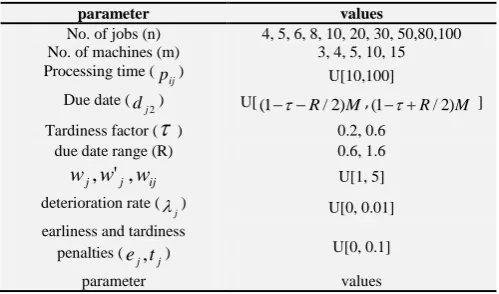
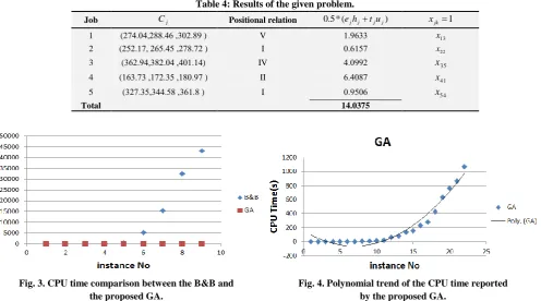
The proposed fuzzy simulation-based genetic algorithm is applied for 22 random type problems with different structures, where each of them is solved 10 times and the best solution was selected. Thus, there were 220 runs in total. For this reason, a personal computer including two Intel CoreTM2 [email protected] processors and 4 GB RAM is used. The considered test problems are solved by using two approaches: the optimal solution approach B&B under the LINGO9.0 software and the proposed fuzzy GA. These approaches are compared with computational time and obtained objective function values. The associated computational results are shown in Tables 5. As you can see in table 5, the proposed fuzzy GA is very suitable in having acceptable computational time and in finding the best solutions. Also, table 5 demonstrates that B&B algorithm finds the global optimum solution of the small-sized problems in a short time. However, some of the problems cannot be solved in reasonable time. For the first 8 given test problems (small-sized problems), global optimum solutions were obtained after the implied computational time. No global optimum solution was obtained for medium and large-sized problems, even after number of hours. This fact reveals that a meta-heuristic approach is needed to tackle these problems. CPU times of the proposed fuzzy GA and the B&B is compared and illustrated in Fig. 3. However, as you can see in Fig. 3, these CPU times are not obviously comparable. The exponential trend of the B&B's CPU time by increasing the size of test problems is tangible. On the contrary, as can be observed in Fig. 4, the CPU time reported by the proposed fuzzy GA shows a polynomial behavior by the increase of the test problems size.

6. CONCLUSIONS AND FUTURE WORK

algorithm in having appropriate computational time has been proved. Future studies can focus on the other features of deterioration such as non-linear functions. In addition,

designing other meta-heuristic approaches may be devised for the further works.

Table 2: The values of controllable parameters for each type of numerical instance.

Type τ R Range of dj2

a 0.2 0.6 [0.5M, 1.1M]

b 0.2 1.6 [0, 1.6M]

c 0.6 0.6 [0.1M, 0.7M]

[image:7.595.53.536.135.291.2]

d 0.6 1.6 [0, 1.2M]

Table 3: sample problem data.

j

t

j

e j



j

d j

p_3,

~ j

p2,

~

j

p

1,

~

Job

0.01336 0.063443

0.005981 (270.95, 286.00, 301.05, 316.11)

(20.36, 21.43,22.50) (86.95, 91.52,9610)

(79.16, 83.33,87.49)

1

0.005929 0.054123

0.003949 (197.11, 208.06, 219.01, 229.96)

(87.80, 92.42, 97.04)

(45.56, 47.96, 50.36) (21.63,22.77,23.91)

2

0.063437 0.074421

0.007356 (328.15, 346.38, 364.61, 382.84)

(33.18, 34.92, 36.67) (12.22, 12.86, 13.51)

(69.87, 73.54,77.22)

3

0.079188 0.024753

0.003421 (278.59, 294.07, 309.54, 325.02)

(64.76, 68.17, 71.58) (47.60, 50.10, 52.61)

(51.37, 54.08, 56.78)

4

0.009199 0.085104

0.00201 (270.39, 285.41, 300.43, 315.45)

(52.76, 55.54, 58.31) (31.31, 32.96, 34.61)

(73.73, 77.61, 81.49)

[image:7.595.45.542.313.589.2]

5

Table 4: Results of the given problem.

1  jk

x )

( * 5 .

0 ejhjtjuj Positional relation

j

C

Job

13

x

136933 V

(204374,2..349 ,3723.6 ) 1

22

x

739150 I

(252310,295345,20.302 ) 2

35 x 437662

IV (392364,3.2374 ,471314)

3

41

x 9347.7

II (193303 ,102335 ,1.7360 )

4

54 x 736579

I (320335,34435. ,3913. )

5

[image:7.595.57.545.637.763.2]

14.0375 Total

Table 5: Comparison between results of the model solved by B&B with the proposed GA.

No.

Problem information Fuzzy B&B Fuzzy GA

No. of jobs No. of

machines type Best solution Optimal solution

Mean CPU

timea Best solution

Mean CPU timea

1 4 3 c 49.04 49.04 00:00:03 49.04 00:00:01

2 4 4 a 64.93 64.93 00:00:11 64.93 00:00:01

3 5 3 c 81.12 81.12 00:02:19 81.12 00:00:03

4 5 4 d 200.17 200.17 00:03:08 200.17 00:00:04

5 6 3 a 126.6 126.6 00:07:34 126.6 00:00:05

6 6 4 b 210.7 210.7 01:27:21 210.7 00:00:06

7 8 3 d 278.8 278.8 04:15:51 278.8 00:00:06

8 8 4 c 474.4 474.4 09:02:33 474.4 00:00:09

9 17 3 c 463.76 - 12:00:00 262.3 00:00:12

10 17 4 a 1515.43 - 12:00:00 918.3 00:00:15

Fig. 3. CPU time comparison between the B&B and the proposed GA.

11 15 5 b 2341.12 - 12:00:00 1814.74 00:00:23

12 15 15 d 4513.43 - 12:00:00 3262.71 00:01:03

13 20 5 a - - 20:00:00 5476.58 00:01:24

14 20 15 c - - 20:00:00 27126.48 00:02:18

15 30 5 c - - 20:00:00 8083.81 00:02:37

16 30 15 b - - 20:00:00 37214.17 00:03:52

17 50 5 d - - 30:00:00 12554.75 00:04:03

18 50 15 b - - 30:00:00 54131.56 00:07:11

19 80 5 a - - 30:00:00 26641.48 00:10:33

20 80 15 b - - 30:00:00 107797.19 00:12:41

21 100 5 d - - 30:00:00 35509.83 00:14:23

22 100 15 a - - 30:00:00 115788.60 00:17:48

a _{Computational time (hour: minute: second).}

7. REFERENCES

[1] Bank, M., Fatemi-Ghomi, S.M.T., Jolai, F., Behnamian, J., 2012. Application of particle swarm optimization and simulated annealing algorithms in flow shop scheduling problem under linear deterioration, Advances in Engineering Software 47:1–6.

[2] Gupta, J.N.D, Gupta, S.K., 1988. Single facility scheduling with nonlinear processing times, Computers & Industrial Engineering 14: 387–393.

[3] Kononov, A., Gawiejnowicz, S., 2001. NP-hard cases in scheduling deteriorating jobs on dedicated machines. Journal of the Operational Research Society 52 (6): 708–717.

[4] Mosheiov, G., 2002. Complexity analysis of job-shop scheduling with deteriorating jobs. Discrete Applied Mathematics 117: 195–209.

[5] Wang, J.B., Xia, Z.Q., 2006. Flow shop scheduling with deteriorating jobs under dominating machines. Omega, 34, 327–336.

[6] Ng, C.T., Wang J.B., Cheng, T.C.E., Liu, L.L., 2010. A branch-and-bound algorithm for solving a two-machine flow shop problem with deteriorating jobs. Comput Oper Res 37:83–90.

[7] Bank, M., Fatemi-Ghomi, S.M.T., Jolai, F., Behnamian, J., 2012. Two-machine flow shop total tardiness scheduling problem with deteriorating jobs, Appl. Math. Modell, doi: 10.1016/j.apm. 2011.12.010.

[8] Balin, S., 2011. Parallel machine scheduling with fuzzy processing times using a robust genetic algorithm and simulation, Information Sciences 181:3551–3569.

[9] Anglani, A., Grieco, A., Guerriero, E., Musmanno, R., 2005. Robust scheduling of parallel machines with sequence-dependent setup costs, European Journal of Operational Research 161:704–720.

[10] Tran, L., Duzkstein, L., 2002. Comparison of fuzzy numbers using a fuzzy distance measure, Fuzzy Sets and Systems 130: 331–341.

[11] Ruiz, R., Stützle, T., 2008 An iterated greedy heuristic for the sequence dependent setup times flow shop problem with makespan and weighted tardiness objectives. European Journal of Operational Research 187(3): 1143–59.

[12] Fortemps, P., Roubens, M., 1996. Ranking and defuzzification methods based on area compensation. Fuzzy Sets and Systems, 82, 319–330.

[13] Wu, H.C., 2010. Solving the fuzzy earliness and tardiness in scheduling problems by using Genetic algorithms. Expert Systems with Applications 37: 4860–4866.

[14] Lin, S.W., Ying, K.C., Lee, Z.J., 2009. Metaheuristics for scheduling a non-permutation flow line manufacturing cell with sequence dependent family setup times, Computers and Operations Research, 36(4): 1110–1121.

[15] Kurz, M.E., Askin, R.G., 2004. Scheduling flexible flow lines with sequence dependent setup times, European Journal of Operational Research 159 (1): 66–82.

[16] Tavakkoli-Moghaddama, R., Taheri, F., Bazzazi, M., Izadi, M., Sassani, F., 2009. Design of a genetic algorithm for bi-objective unrelated parallel machines scheduling with sequence-dependent setup times and precedence constraints, Computers & Operations Research 36: 3224 – 3230.

[17] Moslehi, G., Mirzaee, M., Vasei, M., Modarres, M., Azaron, A., 2009. Two-machine flow shop scheduling to minimize the sum of maximum earliness and tardiness, Int. J. Production Economics 122:763–773.