Comparative Study of Different Path Planning Algorithms: A Water based Rescue System

Comparative Study of Different Path Planning

Algorithms: A Water based Rescue System

S. M. Masudur Rahman Al-Arif, A. H. M. Iftekharul Ferdous, Sohrab Hassan Nijami

Department of Electrical and Electronic Engineering Islamic University of Technology (IUT) Boardbazar, Gazipur – 1704, Bangladesh.

ABSTRACT

There are many countries in the world where water is the main medium for earning livelihood and transportation. Such countries are situated mainly in the over-populated South Asian region. As the water is the meaning of life there; it is also the main reason of threat. Many water borne natural disasters, mechanical failure of manmade water vehicles and sometimes manmade inventions like looting, hijacking put the people in dangerous situation. For rescuing people from being stuck in water, we present a system which can provide a minimum cost, least time rescue operation automatically. We are going to use artificial intelligence (AI) and the concept of mobile robots to represents the proposed system. To find the minimum cost and time, we will consider all available search algorithms. We will also present a comparative result, to find out the most suitable algorithm that can provide us the best results.

General Terms

Path Planning, Rescue System, Algorithms.

Keywords

Artificial Intelligence, Mobile Robot, A-Star, Dijkstra.

1.

INTRODUCTION

To rescue people from a water affected area generally two types of approaches are applied: one is air vehicles; another is water (automatic boat). To conduct an air based rescue operation is too expensive to bear in the South Asian developing countries. So, in the view of economic conditions of these countries, automated water vehicles show better efficacy.

In this paper we are going to present a real prototype of an automated rescue system. Artificial Intelligence (AI) is applied on the Mobile Robot to perform this rescue operation. For a mobile robot path planning is one of the most important things. In this paper we will plan the path for the robot using four different search algorithms. All algorithms used here are very common and popular to the researchers.

Firstly we will present the background work done to propose our design. Then the systems will be discussed. After the design is proposed; all used algorithms will be discussed. Then the simulation results will be revealed and finally we will compare all the results to find out the best algorithms.

2.

BACKGROUND

The field of robotics is closely related to AI. Intelligence is required for robots to be able to handle such tasks as objects manipulation and navigation, with sub-problems of localization (knowing where you are) mapping and motion

planning. Different artificial intelligence (AI) techniques are used to provide the robots with intelligence and flexibility so that it can operate in dynamic environments and in the presence of uncertainty. Those techniques belong to three areas of artificial intelligence: Learning, Reasoning and Problem solving. A number of researchers have considered intelligent robotic systems. There are several research works in the area of using robot as rescue system.

An intelligent autonomous control method is proposed for operated robotic system [1]. Multi-sensor is used in tele-operated robotic system to obtain the environment states and the sensory information is fused into different level autonomous controller to meet the need of the change of environment. A sensor based network system for the rescue robot working under a disaster situation is also presented in a work [2]. Here a network system is proposed and an algorithm for a rescue robot to obtain its position under collapsed area is also considered.

A lot of other works are going on about different algorithms that we are going to compare here. Dijkstra algorithm is a very commonly used algorithm. Researchers are working around the world to improve this algorithm more and more [3], [4], [5]. Here in this paper we will compare Dijkstra algorithm with others to find out the most suitable path for rescue operation. A-Star (A*) Algorithm is also very useful for search and rescue operations [6]. Works are going on around the world to make an efficient hardware engine for this algorithm [7] and to use this algorithm in hazardous environment [8].

3.

THE PROPOSED SYSTEM

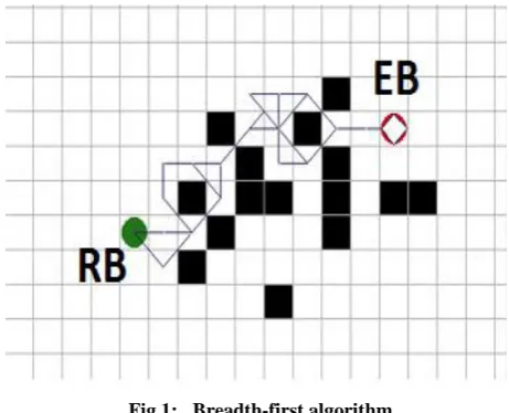
In the system there will be Base Station (BS), Endangered boat (EB) and Rescue Boat (RB). Primarily three rescue boats (RB) are considered to take part in rescue operation in the Endangered boat (EB) and to rescue people to a safe place. There will be a sensor in EB and when EB falls in danger, it will send a signal to the Base station (BS). This signal will have the location and other necessary information. After receiving EB’s signal, BS will find out which RB is the nearest to that EB and will send signal to that RB to perform rescue operation and hence that RB reach to that EB and rescue the victims.

This process will ensure the minimum cost, minimum rescue period and it will keep other RB free so that they can perform another operation if needed.

4.

PATH PLANNING ALGORITHMS

of real-time motion planning is dependent on the accuracy of the map, on robot localization and on the number of obstacles. Topologically, the problem of path planning is related to the shortest path problem of finding a route between two nodes in a graph [9]. The most known algorithms for the shortest path problem are: The graph search algorithm, Breadth-first algorithm, Dijkstra algorithm and A* (A Star) algorithm. In this paper, all these algorithms are summarized and simulated to find a suitable algorithm for our rescue operation. The advantages and disadvantages of different algorithms are defined and experiments for the comparison of the algorithms on various type grid based maps are performed. Some assumptions are taken into account before starting. The map used is a real map which is divided into same size square cells. The ability of traversing is accepted 900 and 4-adjacent traversable neighbor’s is considered [10].

4.1

The Graph Search Algorithm

The graph search algorithms are based on node-edge notation but this notation lacks when a system like GPS gets an image frame, converts it to a map matrix and uses this map matrix as the grid based map. In these situations using matrix notation gives the advantage of simplicity and comprehension.

4.2

The Breadth-First Algorithm

Breadth-first algorithm works with the method branching from the starting cell to the neighbor cells (just traversable cells), (untraversable cells and cells out of boundaries are discarded) until the goal cell is found.

Fig 1: Breadth-first algorithm

Every traversable neighbor cell is added to an array which is called OPEN LIST. OPEN LIST is the array of neighbor cells which must be reviewed in order to find the goal cell. OPEN LIST elements are reviewed if one is the goal cell or not. The steps of breadth-first algorithm can be listed as follows:

i. Define the starting and goal cells. ii. Load the map matrix.

iii. Add the starting cell to OPEN LIST. iv. Add the neighbor cells to OPEN LIST. v. If OPEN LIST is empty, no possible path.

vi. If goal cell is added to OPEN LIST, define the PATH using map matrix. Else compute the cost of neighbor cells.

vii. Pull out the reviewed cells from OPEN LIST. viii. Go to step iv.

4.3

The Dijkstra Algorithm

This algorithm is like Breadth-first algorithm but adds the computation of different cost cells (not only the shortest path but also the lowest cost path). In this algorithm, again the neighbor cell array OPEN LIST exists. Like the previous algorithm here the steps are:

i. Define the starting and goal cells. ii. Load map matrix.

iii. Add the starting cell to OPEN LIST.

iv. Add the neighbor cells to OPEN LIST compute the costs, record their parent cell to PARENTS. v. If OPEN LIST is empty, no possible path.

vi. If goal cell is added to OPEN LIST define the PATH using PARENTS matrix. Else go on. vii. If neighbor cell is added OPEN LIST before find its

new cost and compare to its old cost. If it is lower, update the cost and PARENTS matrix.

viii. Pull out the reviewed cells from OPEN LIST. ix. Go to step iv.

4.4

A-Star (A*) Algorithm

This is the most common and efficient used algorithm in shortest path finding problems. This algorithm has two list arrays:

i) OPEN LIST ii) CLOSED LIST.

OPEN LIST does the same work and CLOSED LIST holds the cells that have to be saved. Again first the neighbors of the starting cell are added to the OPEN LIST. And again these cells are reviewed according to their costs. But this time two cost functions exist. G = cost of moving from the starting cell to the current cell. H = cost of moving from the current cell to the goal cell. Cost at any point n, F(n)=G(n) + H(n). First the G cost function is the cost of moving from the starting cell to the current cell and the H cost function is the cost of moving from the current cell to the goal cell. The G cost function can be computed but the H cost function can just be estimated. That’s why this cost function is called heuristic cost function. There are several methods for this estimation. For 4-adjacent traversable cells Manhattan method is the most used method.

H(currentcell)=abs(currentX-goalX)+abs(currentY-goalY) This method directs the search to the goal cell. The total cost function F = G + H is the comparison criterion for the cells. OPEN LIST has to be sorted and in addition as the comparison criterion the F cost array has to be sorted. The parents of the neighbor cells are stored in PARENTS array. Again in this algorithm if the cell exists in OPEN LIST its new cost must be compared to the old cost. If it is lower the cell becomes the parent and G and F costs must be re-computed. The reviewed cells are placed in the CLOSED LIST. Again after the goal cell is added to OPEN LIST, following the parent cells gives the shortest path. If the OPEN LIST is empty at anytime, it means that there is no possible path. The algorithm can be summarized as follows:

iii. Add the starting cell to OPEN LIST. iv. Add the staring cell to CLOSED LIST.

v. Add the neighbor cells to OPEN LIST: - If traversable; - If not in OPEN LIST before; - If not in CLOSED LIST; With the order compute G, H and F cost function values. Record the parent to PARENTS matrix. Locate the F cost function value in the right place- If in OPEN LIST before; Compute the G cost function value. If it is better than the old value, chance the parent with this parent in PARENTS matrix. Update G and F cost functions.

vi. If OPEN LIST is empty, no possible path.

vii. If the goal cell is added to OPEN LIST define the PATH using PARENTS matrix.

viii. Find the lowest cost neighbor cell. Add it to CLOSED LIST and continue the search on this cell. ix. Pull out the reviewed cells from OPEN LIST. Go to

step v.

5.

MULTI-GOAL CELLS

The above presented algorithms are applicable only for one starting cell - one goal cell. But in reality one starting cell-multiple goal cells scenario like the figure below is most common. So a RB may have to rescue more than one EB (rare case). There is no order between the EB’s. In such cases all possible paths have to be calculated. First we need to find n! Paths between the points (n = number of goal points, |SG1|, |SG2 |, |SG3| , |G1G2| , |G1G3| , |G2G3|) and then the shortest path from starting point to multi-goal points (all points have to be visited once) have to be selected.

Fig 2: One starting-multi-goal points (S: starting point, G1-G2-G3 : goal points)

6.

RESULT AND SIMULATION

All algorithms are simulated for both cases: i. One starting cell - one goal cell and ii. One starting cell- multi goal cells.

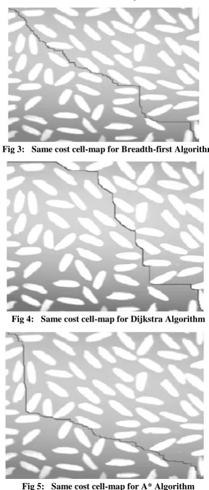
At first the algorithms are compared for one starting cell-one goal cells. As mentioned before, the Breadth-first algorithm is lack of computing different cost cells. So two maps are used

for this case. One with same cost cells (Breadth-first, Dijkstra, A*) and One for different cost cells (Dijkstra , A*).

Fig 3: Same cost cell-map for Breadth-first Algorithm

Fig 4: Same cost cell-map for Dijkstra Algorithm

Fig 5: Same cost cell-map for A* Algorithm

The map is a photo from MATLAB Image Processing Toolbox. First it is converted to a map matrix then the path is computed from this matrix. The dimension of the matrix is 256*256 cells. The white cells are assumed as the obstacles and the grey cells are assumed as traversable cells. The left top side is assumed (0,0). The coordinates of the starting cell and goal cell are (2,2) and (255,255). The black curve in the figure is the path found.

Table-1 lists the comparison of algorithms for CPU time, the sum of the cells, the cells visited, and the path cells. It can be seen that although the Breadth-first algorithm visits more cells, its CPU time is better than Dijkstra and A*.

Table 1. Comparison of algorithms for same cost cell-map

Algorithm CPU Time (s) Sum of the cells visited

Sum of the path cells

Breadth-First 1.078 43002 506

Dijkstra 2.625 43004 506

A* 2.297 25134 506

Fig 6: Different cost cell map for Dijkstra

Fig 7: Different cost cell map for A*

Fig 6 and Fig 7 show the maps with different cost cells and the paths for the algorithms. Again the dimensions are 256*256 cell and the coordinates of starting cell and goal cell are (3, 3) and (255, 255).This map is created by hand. Two layers with costs 60 and 20 surround the big obstacles and the empty spaces in the map are filled with randomly generated different cost cells. They were shown with cells with white and tones of gray according to the cost. (White: 10, white-like grey: 20, grey: 30, darkgrey: 40, black-like grey: 60). The black curve shows the path found. Table-2 lists the comparison of algorithms for CPU time, sum of the cells, the cells visited, the path cells and cost sum of the path cells. It can be seen from the table that A* algorithm doesn’t give the shortest and the lowest cost path. The quality of A* algorithm depends on the quality of the heuristic cost function H. If H is close to the true cost of the remaining path, A* algorithm guarantees finding the shortest and lowest cost path. In other condition A* gives no guarantee but it is still efficient.

Table 2. Comparison of algorithms for different cost cell-map

Algorithm CPU Time _(s) Sum of the cells visited

Sum of the path cells

Cost sum of the path cells

Dijkstra 2.097 35280 537 6970

A* 1.718 26990 545 7000

Table-2 shows that the cost sum of the path cells found by A* is 0.4 % higher than Dijkstra’s but it is 21.9 % faster and it needs 30.7 % less memory according to the sum of the cells visited. In the second group algorithms are compared for one starting-multi goal cells. Again the map with different cost cells is used. Three goal cells are defined on the map. The coordinates of starting cell and goal cells are given below. S: (3,3) G1: (120,5) G2: (190,140) G3: (70,185)

Fig 8: Maps and path for algorithms

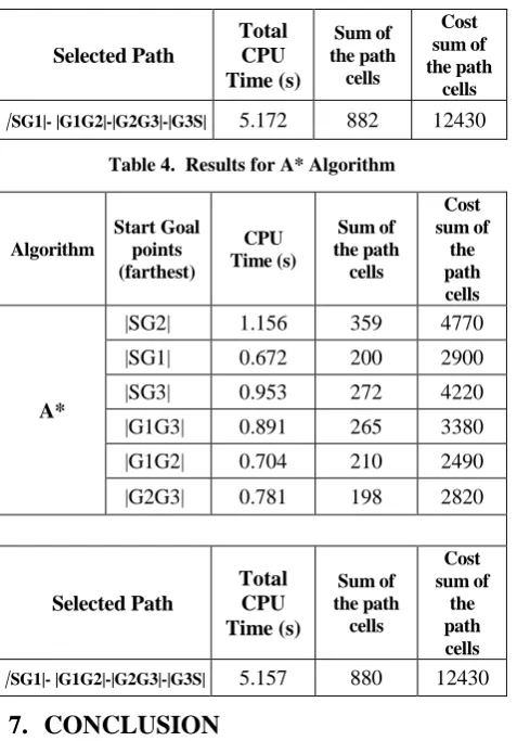
Figure 8 shows the map and the path for the algorithms. Table-3 lists the comparison of algorithms for different start-goal points , CPU times , sum of the path cells cost sum of the path cells and selected path ,total CPU time , sum of the path cells and the cost sum of the path cells. This time A* gives the shortest path. It can be seen that the total CPU times are very close. This result comes from the advantage of computing paths using visited cells. In Dijkstra |SG1|, |SG3| and |G1G2| cells are visited in the previous path and there is no need to re-compute the cells. A* is lack of this advantage but it is still more efficient in computing operations.

Table 3. Results for Dijkstra Algorithm

Algorithm

Start Goal points (farthest)

CPU Time (s)

Sum of the path

cells

Cost sum of the path

cells

Dijkstra

|SG2| 1.453 359 4770

|SG1|* 0.078 198 2900

|SG3|* 0.094 276 4220

|G1G3| 1.594 265 3380

|G1G2|** 0.078 210 2490

|G2G3| 1.875 198 2820

Selected Path

Total CPU Time (s)

Sum of the path

cells

Cost sum of the path

cells

|SG1|- |G1G2|-|G2G3|-|G3S| 5.172 882 12430

Table 4. Results for A* Algorithm

Algorithm

Start Goal points (farthest)

CPU Time (s)

Sum of the path

cells

Cost sum of

the path cells

A*

|SG2| 1.156 359 4770

|SG1| 0.672 200 2900

|SG3| 0.953 272 4220

|G1G3| 0.891 265 3380

|G1G2| 0.704 210 2490

|G2G3| 0.781 198 2820

Selected Path

Total CPU Time (s)

Sum of the path

cells

Cost sum of

the path cells

|SG1|- |G1G2|-|G2G3|-|G3S| 5.157 880 12430

7.

CONCLUSION

This paper presents three path planning algorithms for a mobile robot on grid based map for one starting-one goal cell and one starting-multi goal cells. From the results of the experiments and the inferences from the algorithms some suggestions can be done for path planning for maps with same cost cells, different cost cells and with one starting-one goal and one starting-multi goal cells. For maps with same cost cells, with one starting-one goal cell and multi goal cells, using Breadth-first algorithm is the best if the computational time is the first desire criteria. But if the size of memory is the first criteria using A* can be a better alternative. For maps with different cost cells and with one starting - one goal cell A* is best in computational time and size of memory. But the heuristic function H for A* must be chosen carefully in order to make sure of the shortest and lowest cost path. For maps with different cost cells and with one starting-multi goal cells A* is best in computational time with no guarantee for the shortest path. But it must be noted that Dijkstra, using visited cells advantage especially in enormous multi-goal cells and shortest path guarantee, can be a good choice in these maps. The algorithms use 4-adjacent traversable cells related to the mobile robot. If a mobile robot with more movement abilities is accepted, using 8- and 16- adjacent traversable cells give better results. In the experiments A* uses Manhattan method as the heuristic function. Using other functions may give better results. Choosing the shortest path for multi goal cells using the TSP solving methods can be the next step of this study and it is planned to use real geographical maps instead of the imaginary generated maps.

8.

REFERENCES

[1] Chou Wusheng, Wang Tianmiao, You Song, “Sensor-based autonomous control for telerobotic system,” Proceedings of the 4th World Congress on Intelligent Control and Automation, 2002, vol.3, pp. 2430 - 2434. [2] Miyama, S.; Imai, M.; Anzai, Y.; “Rescue robot

under disaster situation: position acquisition with Omni-directional Sensor”, IEEE/RSJ International Conference on Intelligent Robots and Systems, 2003. (IROS 2003), 27-31 Oct. 2003, vol.3, pp. 3132 – 3137.

[3] Yin Chao, Wang Hongxia, “Developed Dijkstra shortest path search algorithm and simulation”, International Conference on Computer Design and Applications (ICCDA), 2010, 25-27 June 2010, vol.1, pp. 116-119. [4] Hwan Il Kang, Byunghee Lee, Kabil Kim, “Path

Planning Algorithm Using the Particle Swarm Optimization and the Improved Dijkstra Algorithm”, Pacific-Asia Workshop on Computational Intelligence and Industrial Application, 2008. PACIIA '08, 19-20 Dec. 2008, vol.2, pp.1002-1004.

[5] Zhang Fuhao, Liu Jiping, “An Algorithm of Shortest Path Based on Dijkstra for Huge Data”, 6th

International Conference on Fuzzy Systems and Knowledge Discovery, 2009. FSKD '09, 14-16 Aug. 2009, vol.4, pp.244-247.

[6] Xiang Liu, Daoxiong Gong, “A comparative study of A-star algorithms for search and rescue in perfect maze”, International Conference on Electric Information and Control Engineering (ICEICE), 2011, 15-17 April 2011, pp. 24-27.

[7] Woo-Jin Seo, Seung-Ho Ok, Jin-Ho Ahn, Sungho Kang, Byungin Moon, “Study on the hazardous blocked synthetic value and the optimization route of hazardous material transportation network based on A-star algorithm”, 5th

International Joint Conference on INC, IMS and IDC, 2009. NCM '09, 25-27 Aug. 2009, pp. 1499 –1502.

[8] Ma Changxi, Diao Aixia, Chen Zhizhong, Qi Bo, “Study on the hazardous blocked synthetic value and the optimization route of hazardous material transportation network based on A-star algorithm”, 7th International Conference on Natural Computation, 26-28 July 2011, vol.4, pp. 2292 – 2294.

[9] Amerongen, J. van, "Ship Steering", Theme: Control Systems, Robotics and Automation, edited by Unbehauen, H.D. , in Encyclopedia of Life Support Systems, (EOLSS), Developed under the Auspices of the UNESCO, EOLSS Publishers, Oxford, UK , 2003. [10] Donoso-Aguirre, F. et al. “Mobile robot localization

using the Hausdorff distance”, ROBOTICA, Cambridge University Press, vol. 26, pp. 129–141, 2008.

[11] Mata et al. “Object learning and detection using evolutionary deformable models for mobile robot navigation”, ROBOTICA, Cambridge University Press, vol. 26, pp. 99–107, 2008.