Principal Pattern Analysis:
A Combined Approach for Dimensionality Reduction
with Pattern Categorization
T. Kalai Chelvi
Research Scholar, Sathyabama University,
Chennai, India
P.Rangarajan
Professor& Head/IT R.M.K. engineering college
kavaraipettai Tamilnadu, India
ABSTRACT
Over the past decades there has been several techniques found to overcome the data analysis problem in most of the science domains such as engineering, astronomy, biology, remote sensing, economics, consumer transactions etc., It is required to reduce the dimension of the data (having less features) in order to improve the efficiency and accuracy of data analysis. Traditional statistical methods partly calls off due to the increase in the number of observations, but mainly because of the increase in number of variables associated with each observation. As a consequence an ideal technique called Principal Pattern Analysis is developed which encapsulates feature extraction and categorize features. Initially it applies principal component analysis to extract eigen vectors similarly to prove pattern categorization theorem the corresponding patterns are segregated. Certain decisive factors as weight vectors are determined to categorize the patterns. Experimental results have been proved that error approximation rate is very less too it’s more versatile for high dimensional datasets.
Keywords
Principal Component Analysis, Eigen vectors, Dimensionality reduction.
1. INTRODUCTION
In order to mine the surplus data besides estimating gold nugget (decisions) from data involves several data mining techniques. The assessment could be as simple, so as to make decision for particular conditions of company in a share market, or to decide whether a consumer is profitable or not to a particular concern. The dimensionality reduction comes down to almost reducing the number of variables to few category (newly definable) variables (reduce huge dimensions to linear or non-linear combinations of variables, also called reduce variables to category dimensions) or categorizations of huge dimensional spaces into understandable fewer partitioned spaces of category spaces (reduce huge dimensions to category spaces), with appropriate deduction of unusual dimensions, variables, categories, and spaces (also termed outlying variables, outlying categories, and outlying spaces). In addition the trends not attributable to robust decision rules from the data. For instance, in a large credit company the number of variables involved to analyze is in thousands. The ultimate question is whether the individual could be authorized for upgrade of his card to higher priced, better-serviced card with in the franchise. The analysts could use all the following: However based on the purpose, whether we are looking for decision rules out of the data, how easy to interpret, or how robust (less affected by outlying observation
and probability distributional assumptions of data), one may choose the right one. Some guidelines are provided below to that effectwhether we are looking for decision rules out of the data,
1) How easy to interpret,
2) How robust (less affected by outlying observations and probability distributional assumptions of data), one may choose the right one.
3) Predicting importance of variable.
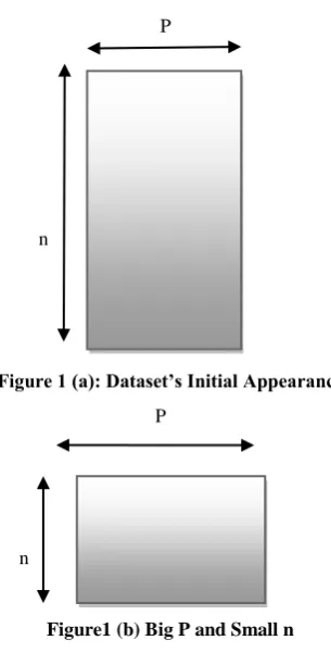
The dimension of the data depends on the number of variables that are measured on each observation.While considering the statistical records data accumulates in an unprecedented speed so Dimensionality reduction is an effective approach for diluting the data. There exists some problems of “Big p Small n”, these are extreme examples of situations where Dimension Reduction (DR) is necessary because the number of explanatory variables p exceeds (sometimes greatly exceeds) the number of samples [11]. While approaching from a statistical point of view it is desirable that the number of examples in the training set should significantly exceed the number of features used to describe those examples (Figure 1(a)). Moreover the number of examples increases exponentially with the number of features, if inference is to be made with the data. If this is not the case, accordingly only the real high-dimension occupies a manifold in the input space so the implicit dimension of the data will be less than the number of features p. This is expressed in Figure 1(b) can be still analyzed.
Traditional algorithms however, are applied in machine learning and pattern recognition applications which are often susceptible to the well-known problem of the curse of dimensionality. In the assessment of performance of a given learning algorithm as a data pre-processing step, or as part of the data analysis to simplify the data model it is referred as the degradation. Crucially this involves the identification of a suitable low-dimensional representation for the original high-dimensional data set. While working with this reduced representation, tasks such as classification or clustering can often yield more accurate and readily interpretable results, further the computational costs may also be significantly reduced.
Hereby the keen impulse of dimension reduction is encapsulated,
2. For a number of learning algorithms, the training and/
or classification time increases directly with the number of features.
3. Noisy or irrelevant features can have the same influence on classification as predictive features, so they will impact negatively on accuracy.
4. Things look more similar on average other than the abundant features used to describe them; Hence the outcome after dimensionality reduction is represented in figure 2.
P
n
Figure 1 (a): Dataset’s Initial Appearance
P
n
Figure1 (b) Big P and Small n
[image:2.595.367.468.89.353.2]On the other hand still there is an ever growing needs for techniques related to the dimensionality reduction and classification. A novel algorithm called Principal Pattern Analysis algorithm (PPA) is presented in our proposed work. The work partially implements Principal Component analysis algorithm and then employs the principal pattern analysis algorithm, consequently evaluating the feature patterns .The figure 2 stochastically expresses the reality of dimensionality reduction.
Figure 2: Dimensionality Reduction
The rest of the paper is organized as follows. Section 1 discusses the related works in Dimensionality reduction techniques; Section 2 presents the Basic Credentials related to our proposed work. The summarization of our proposed system is exemplified in Section 3; Experimental results are delineated in Section 4. This paper is circumscribed with conclusion in Section 5.
2. Related Works
There are several implementations of dimensionality reduction platforms, providing various levels of functionality either regarding on the unsupervised or supervised data.
Traditionally, the missing value problem in PCA is first studied by Dear (1959), who only used one component and one imputation iteration (see below). It is based on the minimum mean square error formulation of PCA which is introduced by Young (1941). Wiberg (1976) first suggested directly minimizing the mean-square error of the observed part of the data. An algorithm by de Ligny et al. (1981) already worked with up to half of the values missing. The missing values problem using a multivariate normal distribution has been studied even earlier than using PCA, for instance, by Anderson (1957). More historical references can be found in the book by Jolliffe (2002).
[image:2.595.88.241.197.498.2]that will generalize well, and adopts a subset of non zero
weighted variables found by the linear models to produce a final nonlinear model.
The authors in [1] have suggested a method based on PCA. They have implemented Multi-level Mahalanobisbased Dimensionality Reduction (MMDR). In the technique of Multi-level Mahalanobis-based Dimensionality Reduction, it is able to reduce the number of dimensions while keeping the precision high, and handles large datasets effectively. In order to index the data points in different reduced subspaces the extended iDistance metrics is used.
On the other hand some economical model-based schemes are proposed by author [5]. As it is known that Principal component analysis (PCA) is a data analysis technique that can be traced back to Pearson, where some of the data values are missing, and it is shown that there are many features which are usually associated with nonlinear models, such as over fitting also resulting in bad local optimal solutions. For the sake a probabilistic formulation of PCA, a good foundation for handling missing values is exhausted, consequently formulas are wrapped for doing that. There are several problems and traditional algorithms for PCA in case of high dimensions along with the very sparse data also over fitting are very slow. As a result a novel fast algorithm is discovered by the authors of whom it is extended to variation in Bayesian learning.
Still extending the work of [14], an enhanced novelized approach is presented for dimensionality reduction along with pattern classification.
This algorithm gently improves salient features for the problem concerned.
1. The original high-dimensional representation of data is significantly reduced to a lower-dimensional compact representation.
2. Projects the data in the least square sense– it captures big (principal) variability in the data and ignores small variability.
3. Eliminates the unwanted noise in the data.
4. Provides a contemporary methodology for feature extraction.
5. Affords a good strategic decision making scenarios via the pattern classification.
3.
BACKGROUND
Generally the dimension reduction is the process of reduction of concentrated random variables where it can be divided into feature selection and feature extraction.
3.1 Feature Selection
Feature selection, too accessed as variable/attribute selection. Feature reduction, is the technique to construct robust learning models by selecting the subset of relevant features. Alternatively feature selection also helps to acquire better understanding about their data in addition it helps to identify the important features and their relation with each other.
Feature selection helps to improve the performance of learning models by banishing the unwanted and repeated features from the data,
Allaying the effect of the curse of dimensionality. Elevating generalization efficiency.
Rapiding the learning process. Enhancing model interpretability.
3.2 Feature Extraction
Feature extraction is an exceptional form of dimensionality reduction. It is needed when the input data for an algorithm is too large to be processed and it is suspected to be notoriously redundant (much data, but not much information) then the input data will be transformed into a reduced representation set of features (also named features vector). By the way of explanation transforming the input data into the set of features is called feature extraction. The extracted features are carefully chosen. It is expected that the features set will extract the relevant information from the input data in order to perform the desired task using the reduced representation instead of the full size input.
3.3 PCA Brief Outlook
PCA is invented in 1901 by Karl Pearson. Now it is profusely explored as a tool in exploratory data analysis to make predictive models. By means of Eigen value decomposition of a data covariance matrix or singular value decomposition of a data matrix, generally after mean centering the data for each feature the PCA can be worked out. On considering the results of a PCA it is clear that they are commonly conferred in terms of component scores (the transformed variable values corresponding to a particular case in the data) and loadings (the weight by which each standardized original variable should be multiplied to get the component score).
A data matrix, XT, is defined from the training data. Following this the zero empirical mean is computed (the empirical (sample) mean of the distribution has been subtracted from the data set), where each of the m rows representing a different repetition of the experiment, and each of the n columns gives a particular kind results from a particular probe. Computing the XT is often alternatively denoted as X itself. The singular value decomposition (SVD) of X is X = WΣVT, where the m × n matrix W is the matrix of eigenvectors of XXT, the matrix Σ is an m × n rectangular diagonal matrix with non-negative real numbers on the diagonal, and the n × n matrix V is the matrix of eigenvectors of XTX. The number of principal components same as original variables is given by the PCA transformation that preserves dimensionality and this is represented as,
𝒀𝑻= 𝑿𝑻𝑾 = 𝑽∑𝑻𝑾𝑻𝑾 = 𝑽∑𝑻
When m < n – 1 and V is not uniquely defined. Since W (by the delineation of SVD of a real matrix) is an orthogonal matrix, each row of YT is simply a rotation of the corresponding row of XT. The first column of YT is composed of the "scores" of the cases in regards with the "principal" component; while the next column is with the "second principal" component, and so on.
In order to bring more reduced-dimensionality representation,
X can be projected down into the receded space defined by only the first L singular vectors,
Where ΣL=IL×M Σ, IL×M and the L×M represents the
rectangular identity matrix. The matrix W of singular vectors of X is equivalently the matrix W of eigenvectors of the matrix, of observed co variances C = X XT,
Projecting points in the Euclidean space, the first principal component corresponding to a line passes through the multidimensional mean and minimizes the sum of squares of the distances of the points from the line. The second principal component corresponding to the same concept after all correlation with the first principal component has been subtracted out from the points. The singular values (in Σ) are the square roots of the Eigen of the matrix XXT. Each eigenvalue is proportional to the portion of the "variance" (more correctly of the sum of the squared distances of the points from their multidimensional mean) that is correlated with each eigenvector. The sum of all the Eigen values is equal to the sum of the squared distances of the points from their multidimensional mean. PCA principally rotates the set of points around their mean in order to align with the principal components. This moves as much of the variance as possible (using an orthogonal transformation) into the first few dimensions.
3.4 Significant Statistics Metrics
Correlation Matrix
A correlation matrix is used for pointing the simple correlations r, among all possible pairs of variables included in the analysis; also it is a lower triangle matrix. The diagonal elements (of 1) are usually omitted.
Bartlett's test of Sphericity
Bartlett's test of Sphericity is a test statistic used to examine the hypothesis that the variables are uncorrelated in the population. In other words, the population correlation matrix is an identity matrix; each variable correlates perfectly with itself (r = 1) but has no correlation with the other variables (r = 0).
Kaiser-Meyer-Olkin (KMO)
KMO is a measure of sampling adequacy, which is an index. It is applied with the aim of examining the appropriateness of factor/Principal Components analysis. High values (between 0.5 and 1.0) indicate that factor analysis befits and their value below 0.5 implies that factor analysis may not be suitable.
Our proposed approach too proceeds by estimating these statistics.
4. PROPOSED SYSTEMIZATION
The scope of this paper is to present ensemble approach for dimensionality reduction along pattern classification. This section presents PPA algorithm and its step by step processing.
Compute the column vectors such that each column is with M rows.
Locate the column vectors into single matrix X of which each column has M x N dimension. The empirical mean EX is
computed for M x N dimensional matrix.
Subsequently the correlation matrix Cx is computed for M x
N matrix.
Consequently the Eigen values and Eigen Vectors are calculated for X.
By hindering the estimated results, the Principal Pattern Analysis algorithm persists by proving the Pattern Analysis theorem.
4.1 Principal Pattern Analysis
For a given Set of Training patterns S there exists two classes of Pattern δ1 and δ2; i.e. S1={Aiε δ1, i=1,2,……N1; Bj ε δ2,
j=1,2,……N2; N1 >N2 also N1 ,N2 < ∞ where Ai and Bj are n
dimensional vectors also δ1 and δ2 (Eigen measures /Where δ1,
δ2 ε δ) which are linearly inseparable then there exists a
solution weighted vector T which gives linear classification of patterns.
Proof
Assume the two patterns Ai Bj.in which those set is defined to
be a set of real numbers.
Ai .C > 0 where i=1, 2, 3……, N1 .Consider another pattern Bj.
which is defined to be set of real numbers.
Bj. C < 0where j=1, 2, 3……., N2 Rewriting the inequalities
C.Xm > 0, where m=1, 2……N.
At this juncture C indicates the cost vector; here arises a question of how to predict the cost vector. The cost vector value is kept below 0.05. The above said inequalities are computed just to verify the existence of the two sets of patterns.
Xm= Ai for m=i=1, 2, 3……, N1
Xm= -Bj for m=j=1, 2, 3……, N2
Thus a set T= {Xm} is constructed to be patterns which are
linearly undividable.
From the results it is clear that there exists two set of training patterns for both data matrix also the dimensional vectors. Those training patterns are further considered for further processing of pattern classification.
Pattern analysis theorem ends with finally proving two hypothesis for pattern classification.
Hypothesis 1
For the two patterns δ1 and δ2 there exists a weight Matrix
which gives the linear combination of training patterns. To prove this hypothesis we need to prove another hypothesis 2.
Hypothesis 2
For every Ek /k=1, 2….N there exists a constant which
converges to a solution C2 such that C2 →0.
Moreover consider another metrics Yk.; Itis essential to find
the value of Yk. Before computing the value of Yk.; It is
crucial to know about Eigen values and its corresponding Eigen vectors. Data Matrix considered is real; as a result their related Eigen values are real. Let ζk be the Eigen Values and
its corresponding Eigen Vectors be ψk. The Eigen vectors
corresponding to non zero Eigen values are taken to be considered. Consequently assume a constant t where t >0
∝𝒌= σ𝑛𝑘 k 𝑡 ---1 ∑𝒏𝒌=𝟏∝𝒌= 𝒄𝒐𝒏𝒔𝒕𝒂𝒏𝒕 ---2
𝜷𝒌= ∝𝒏𝒌 𝐤 𝛙𝐤 ---3
Assume another constant vector (called decisive vector) γ =0.01 and its corresponding iterative vector is computed by giving a slight increment. Then compute
𝑭𝒌= 𝛄𝒏𝒌 𝐤 𝛙𝐤 ---4 ∑𝒏𝒌=𝟏𝑬𝒌𝛙𝐤 ---5
Where 𝐸𝑘 = γk σk /k represents iterative vectors. Here ∝𝒌 is again taken for computing the error rate which is denoted as
exists a solution converges to 0. The value of γ is taken in
such a way that, itis chosen to be linearly independent vectors when multiplied with the Eigen vectors giving the mutually orthogonal vectors. Equation 4 converges to solution c1; 5
converge to solution c2→0and obviously the hypothesis 2 has
been proved. To evaluate the patterns compute weight matrix
Wk. Wkis computed by having the below equation.
𝑾𝒌 = | 𝑭𝒌− σk|.Thus evaluating the respective features of Wk.; this also provides the patterns which are classified
according to weighted threshold.
6. EXPERIMENTAL RESULT
The proposed algorithm is implemented on having the transactional dataset. The dataset deals about the company’s firm status in the market. The data are trained for further evaluation of reduced dimensions.
Initially the data are organized. The missing responses for the items are replaced respectively by their corresponding mean or zero. On using the correlation, the variables are standardized and the total variance equals the number of variables used in the analysis (because each standardized variable has a variance equal to 1).
On using the covariance matrix, the variable remains in their original metric. However, care must be taken to use variables whose variances are similar. For this reason the correlation matrix are estimated following the Eigen values and Eigen vectors are anticipated. Moreover Kaiser-Meyer-Olkin (KMO) measure is applied for post estimation measure of PCA. This measure is applied for the purpose of qualifying the overall results. On attaining the results, Pattern Analysis Theorem is proved. The experimental results are carried out for having several sample set of data. Pictorial representations for some sample data are endowed here.
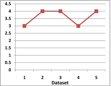
Figure 3: Representation of Patterns acquired w.r.to Dataset
6.1 Impact of Principal Pattern Analysis
On implementing the Pattern Analysis Theorem the results are evaluated. The consequences are represented in the pictorial representations. Foremost figure 3 represents the patterns gained with its corresponding sample datasets. For the first set, patterns (clusters) obtained are three. Similarly 5 patterns are obtained for fifth set of samples.Figure 4 represents the weight matrix obtained and its respective Features. The prioritized Feature is located at the top followed by the next feature. This indicates that the most prioritized feature is 2 proceeding this less prioritized feature is feature 1.
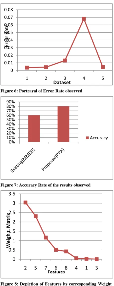
The Experiment is repeated for next dataset. The main concerned feature is judged as feature 2. Next it approaches the 6th feature. In this way the experiment is carried out for all the sample sets. Figure 8 illustrates that the less significant feature is 3 and most significant feature is 2 and so on. The graphical representation in Figure 9 exemplifies the most important feature is 3. On the contrary the most significant feature for sample 5 is predicted as feature 4 from figure 10. From Figure 7 it is observed that accuracy (%) increases for the proposed approach. The accuracy depends on number of missing terms and the plotted dimensional values. All the results obtained so far are depends on the decisive vector. If the decisive vector is 0.01 then the error rate is low, so the accuracy rate is proportional to the decsive factor assumed. It is better to place right decisive factor which should be less than 0.02. Stimulating the decisive factor value results in erroneous situation.
Figure 4: Depiction of Features its corresponding Weight Matrix for Dataset1
Figure 5: Depiction of Features its corresponding Weight Matrix for Dataset2
0 0.5 1 1.5 2 2.5 3 3.5 4 4.5
1 2 3 4 5
Dataset
0 0.5 1 1.5 2 2.5 3 3.5
2 6 7 3 5 8 1 4
Features
W
e
ig
h
t
M
atr
ix
0
0.5
1
1.5
2
2.5
3
3.5
2
5
7
6
8
4
1
3
W
e
ig
h
t
M
atr
[image:5.595.316.545.322.492.2] [image:5.595.54.284.458.636.2] [image:5.595.314.544.518.698.2]Figure 6: Portrayal of Error Rate observed
Figure 7: Accuracy Rate of the results observed
Figure 8: Depiction of Features its corresponding Weight Matrix for Dataset 3
Figure 9: Depiction of Features its corresponding Weight Matrix for Dataset 4
Figure 10: Portrayal of Features its corresponding Weight Matrix for Dataset5
7. CONCLUSION
In this paper a mutual comprehensive solution for the dimensionality reduction ensemble with pattern classification is afforded. The ultimate goal of dimensionality reduction is to rapidly improve the query accuracy and efficiency; simultaneously pattern classification is to select and apply the right pattern at right scenarios. Our proposed approach paves and elucidates above mentioned state of affairs. On proving the PPA theorem dimensionality is reduced on plotting the weight matrix thresholds. On the other hand it is endowed with a priori determination of patterns and thus classified accordingly. In addition this approach reduces the error rate, significant rise in the throughput, reduction in missing of items and finally the patterns are classified. In future still more enhancement of this approach is needed especially concentrating on pattern recognition/classification which is malleable to be applied in other domains such as image processing, forensic studies, gene expression in biological tissue sample, several statistical / stochastic models and ecological communities.
REFERENCES
[1] Jin, H., Ooi, B.C., Shen, H.T., Yu, C., Zhou, A.Y.: An adaptive and efficient dimensionality reduction algorithm for high-dimensional indexing. In: Proc. ICDE. (2003)
[2] Jinbo Bi, Kristin P Bennett, Mark Embrechts, Curt M Breneman, Minghu: Dimensionality Reduction via
0 0.01 0.02 0.03 0.04 0.05 0.06 0.07 0.08
1 2 3 4 5
Dataset
Err
o
r
Ra
te
0% 10% 20% 30% 40% 50% 60% 70% 80% 90%
Accuracy
0
0.5
1
1.5
2
2.5
3
3.5
2
5
7
6
8
4
1
3
W
e
ig
h
t
M
atr
ix
0 0.5 1 1.5 2 2.5 3 3.5
3 4 5 1 7 8 2 6
W
ei
gh
t
M
atr
ix
0 1 2 3 4 5
2 5 8 6 3 7 4 1
W
e
ig
h
t
M
atr
[image:6.595.315.545.82.233.2] [image:6.595.315.546.279.421.2]Sparse Support Vector Machines in Journal of Machine
Learning Research (2003)
[3] Ilin, A. and T. Raiko.” Practical approaches to principal component analysis in the presence of missing values” Journal of Machine Learning Research 11, 2010.
[4] Pearson, K.: On lines and planes of closest fit to systems of points in space. Philosophical Magazine 2(6), 559– 572 (1901)
[5] Jolliffe, I.: Principal Component Analysis. Springer, Heidelberg (1986)
[6] Bishop, C.: Pattern Recognition and Machine Learning. Springer, Heidelberg (2006)
[7] Diamantaras, K., Kung, S.: Principal Component Neural Networks - Theory and Application. Wiley, Chichester (1996)
[8] Alexey Tsymbal, Seppo Puuronen, Mykola Pechenizkiy, Matthias Baumgarten, David Patterson “Eigenvector-based Feature Extraction for Classification”
[9] Haykin, S.: Modern Filters. Macmillan (1989)
[10] Cichocki, A., Amari, S.: Adaptive Blind Signal and Image Processing – Learning Algorithms and Applications. Wiley, Chichester (2002)
[11] Oja, E.: Neural networks, principal components, and subspaces. International Journal of Neural Systems 1(1), 61–68 (1989)
[12] T. Raiko, A. Ilin, and J. Karhunen, “Principal component analysis for large scale problems with lots of missing values,” in Proceedings of the 18th European Conference on Machine Learning (ECML 2007), Warsaw, Poland, September 2007.
[13] Tipping, M., Bishop, C.: Probabilistic principal component analysis. Journal of the Royal Statistical Society: Series B (Statistical Methodology) 61(3), 611– 622 (1999)
[14] M. West. Bayesian factor regression models in the “large p, small n" paradigm. Bayesian Statistics, 7:723{732, 2003.
[15] Grung, B., Manne, R.: Missing values in principal components analysis. Chemometrics and Intelligent Laboratory Systems 42(1), 125–139 (1998).
[16] Bishop, C.: Variational principal components. In: Proc. 9th Int. Conf. on Artificial Neural Networks (ICANN99), pp. 509–514 (1999).
[17] Oba, S., Sato, M., Takemasa, I., Monden, M., Matsubara, K., Ishii, S.: A Bayesian missing value estimation method for gene expression profile data. Bioinformatics 19(16), 2088–2096 (2003)