2017 2nd International Conference on Computer, Mechatronics and Electronic Engineering (CMEE 2017) ISBN: 978-1-60595-532-2
Research on EPSQP Algorithm for Motion Planning of Humanoid Robot
Hua-Zhong LI
1, Zhuo LIANG
2,*and Bo GAO
31,3
Software Department, Shenzhen Institute of Information Technology, No. 2188 Longxiang Road, Longgang District, Shenzhen, 518029/Guangdong, China
2
Shenzhen Middle School, Shenzhen, 518025/Guangdong, China
*Corresponding author
Keywords: Humanoid robot, Motion planning, Enhancing Parametric Sequential Quadratic Programming (EPSQP), Parametric optimum, Dynamics model.
Abstract. Aiming at the instability and low convergence rate caused by complex dynamics, linear constraint and sensitivity to initial configuration state during Sequential Quadratic Programming (SQP) of motion control of humanoid robot solved by parameter optimization method, firstly, establish a general dynamics model for 7 connecting rods of humanoid robot and establish a simplified, multilevel and inverted pendulum model which falls to the ground from the front to the back for falling motion; secondly, introduce a parameter optimization technique to the optimum control of humanoid robot motion, build the optimum control model, adopt a filter for initial configuration state, improve SQP filter algorithm and enhancing technique, propose Enhancing Parametric Sequential Quadratic Programming (EPSQP) algorithm to improve optimizing process and accelerate convergence rate; finally, verify the validity and optimality of EPSQP algorithm proposed in this paper by computer simulation experiment.
Introduction
Humanoid robot is a kind of typical system which features “high-dimensional, nonlinear, complex and intelligent information” and involves in cutting-edge theories and control methods for multi-disciplines including computer, robot and electronic information etc. It carries out various tasks in human’s complex environment, collects the information from different environments and completes various, different and complex motions. It has gradually been a focus concerned by people [1-2].
Motion planning is one of important issues for humanoid robot research [3-5]. Its key techniques include kinematics and dynamics modeling relating to motion planning, joint track and moment control techniques; feasibility analysis, target identification, offline and online planning techniques; multi-sensor information fusion, self-positioning and navigation techniques in path planning; relevant processing techniques[6-12] adopted for optimal object based on decision-making, collaboration and communications processing in task planning and energy consumed by overall motion and motion, time, overall environment stability and other motion planning evaluation system
The typical methods for dynamics modeling of humanoid robot include: inverted pendulum model
[13-15]
and connecting rod model [16-20].
The representative methods for motion control of humanoid robot include: (1) neural network method [21]; (2) fuzzy logic control[22]; (3) genetic algorithm[23]; (4) reinforcement learning[24]; (5) soft computation[25]; (6) parametric control method [26-28]: This method is of good optimizing effect in solving high-dimensional, nonlinear and optimization problems as well as good application in mission attitude control and lunar vehicle soft landing[29].
There are mainly two ways in the research on preventing humanoid robot from falling: (1) how to conduct effective motion compensation to make the robot able to remove the unstable state outside and prevent falling; (2) how to control falling motions to minimize the damage against the humanoid robot.
Parametric motion control method is adopted in this paper. However, this method aims at the instability and low convergence rate caused by complex dynamics, linear constraint and sensitivity to initial configuration state during Sequential Quadratic Programming (SQP) of motion control of humanoid robot solved by parameter optimization method. In view of this, this paper firstly researches the general dynamics modeling method for humanoid robot and focally researches falling dynamics, simplified and inverted pendulum model. Secondly, EPSQP algorithm is proposed based on parametric control and enhancing technique to conduct optimum control for falling motion and optimize ground impact, ground contact position and stability after falling when humanoid robot contacts the ground. Finally, the validity and optimality of EPSQP (motion control algorithm) proposed in this paper is verified by computer simulation experiment.
Dynamics Model for Humanoid Robot
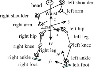
[image:2.612.229.382.335.446.2]The system model for typical humanoid robot (HR) is shown in Fig.1. Each leg of humanoid robot has 6 DoFs (including 3 hip joints, 1 knee joint and 2 ankle joints). Each upper limb has 3 DoFs (including 2 shoulder joints and 1 elbow joint). The head is fixed on the body as a part of the body.
Figure 1. System model for humanoid robot.
Walking motion model of humanoid robot can be abstracted to one 7-connecting-rod mechanism
[16]
and simplified as multilevel and inverted pendulum [17].
Suppose the mass of each connecting rodmiconcentrates in the center of connecting rod, rotational inertia of connection rodiisIi,θi is inclined angle between connecting rod and ground perpendicular line and qiis inclined angle between the two adjacent connecting rods i-1 and i (namely rotational angle of rotating joints). Taking the tiptoe of left supporting leg of humanoid robot as the original point, the expression for barycenter coordinates of each connecting rod(xi,zi)(i=1,…,7) can be obtained through the geometrical relationship. Then, total kinetic energyE (1) and V (2) for humanoid robot system can be obtained:
] )
(
[ 2 2 12 2
7 1 2
1
i i i i i
i m x z Iq
E=
∑
+ += 2q J( )q 1 T θ
= (1)
∑
∑
= = == 7
1 7
1 i i
i migzi N gci
V θ (2)
Where, J(
θ
)=[Lijc(θi−θj)]i×j∈7×7is mass inertia matrix. SupposeL=E−Vis mechanical energy ofhumanoid robot, τi is generalized force corresponding to generalized coordinatesθi of the joint, then dynamics equation (3) can be obtained according to Lagrangian dynamics d dt
(
∂L ∂θi)
−∂L ∂θi =τi (i=1,,7):x y z
G
∑CM
N ft
head right shoulder
left shoulder left arm right arm
right hip
left hip Waist
left knee right knee
left ankle right ankle
left leg right leg
u H
θ
G
θ θ θ
C
θ θ
D( )+ ( ,)+ ( )= T (3) Where, D(θ)=J(θ)=[Lijc(θi−θj)]i×j∈7×7 is inertial matrix, ( , )=[Lijs(θi−θj)θj]i×j∈7×7
θ θ
C is first order
differential matrix consisting of viscous resistance, Coriolis force and centrifugal force,
1 7 ] [ )
( = i i×j∈×
i gc
N θ
θ
G is gravity-related matrix, and u=
[
u1 un]
T is driving moment driving moment for each joint.The barycenter velocity of humanoid robotυCMand the speed of each jointθcan be expressed in Formula (4):
[
]
J( )
θθ υT = CM CM CM T =CM x ,y ,z (4)
Acceleration vector of barycenter velocityaCM(5) can be obtained by conducting differential for barycenter velocity vectorυCMin Formula (4):
=
= T
CM T
CM υ
a
[
xCM,yCM,zCM]
T =J( )
θθ+J(θ,θ)θ (5)Where, Formula (5) θ=
[
θ1, , θn]
T is acceleration vector of robot joint angle. Formula (6) is as follows:θ θ θ
J
θ
J a
θ
J
θ
= ( )−1 T − ( )−1 ( , )
CM (6)
[image:3.612.230.384.369.487.2]After acceleration of barycenter is obtained by Formula (5), the acceleration of each joint angle can be calculated by Formula (6).
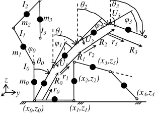
Figure 2. Motion model for front falling.
Aiming at falling motion modeling of humanoid robot, it can be divided into front falling and back falling. As for back falling, ground contact point and center of gravity are very close each other. Humanoid robot can be simplified as a 1-level and two-dimensional inverted pendulum model. Its dynamic equation can be described with differential equation [15]:
= −
+
= +
−
M gr
r r r
M f g
r r
/ sin 2
/ cos
2 2
τ
θ
θ
θ
θ
θ
(7)
Where, ris perpendicular distance from barycenter to ground,
θ
is angle of falling rotation, f is elastic force of controlling falling, different elastic forcesf can generate different centre-of-gravity paths,M is total mass of humanoid robot,τ
is rotating moment, and g is gravitational acceleration ofthe point where humanoid robot is located.
Front falling is a very complex process which can be divided into two sub-processes of ground contact by knee and ground contact by hand. In this paper, it is abstracted as a 4-level inverted pendulum model (shown in Fig.2). Dynamics model (8) [13]can be obtained for the falling processing
of humanoid robot according to Lagrange equation j j j
Q D T
dt d
= ∂
∂ −
∂ ∂
θ
θ ( j=1,2,,k):
x y
z
(x0,z0) )
(x1,z1) )
(x3,z3) )
(x4,z4) ) (x2,z2)
)
θ0
φ0
θ1
φ1
θ2 θ3
φ3
φ2
m0 m1
m2 m3
r0 R0 I0 I1
I2
I3
U1 U2
U3
r1 R1
r2 R2 r3
u
D
θ
C
θ
B
θ
A+ 2+ sin = (8) Where, A, B, C and D are the coefficients for 4-level inverted pendulum model calculated according to Lagrange equation. T
q q q
q, , , ]
[ 1 2 3 4
=
q , T
] , , ,
[θ1θ2 θ3 θ4
=
θ , q=Kθ , A={Lijc(θi−θj)}, }
{ ( )
j i
s Lij θ−θ =
B , C =-diag( gG ), D=KTKm G=αTM , M=[m1,m2,m3,m4]T ,
) (
) (
3 1
2 3
1
j i
j i
I M
M L
n n ni i
n n ni nj
ij
= ≠
+ =
∑
∑
= =
α α α
,I=[I1,I2,I3,I4]T,θn is inclined angle between No.njoint and ground
perpendicular line, qnis relative inclined angle of No.njoint, Inis rotational inertia of No.njoint, un
is moment input of No.njoint, andmiis mass for each joint of robot.
When the knees or hands of humanoid robot contact the ground, its aggregate momentum is
j j mjc
P
∑
=
= 4
1 , in which cjis speed of barycenter of No. jinverted pendulum that can be calculated bycj =vj+
θ
j×(
Rjcj)
. vj ,θ
j andRj are speed, angular speed and attitude of No. j inverted pendulum. cjis barycenter relative to local coordinate system. After the robot contacts the ground, the instant angular momentum can be obtained from the following equation (9):j T
j j j j j
j c P
L = × +R I R ω (9) Where, cjis barycenter of No.jconnecting rod, Ijis inertia tensor of No. jconnecting rod relative to local coordinate system. Therefore, angular momentum equation (10) for falling of humanoid robot can be obtained according to equation (9):
[
− + −]
+Iθ = c( c j) c( c j)j M x x x z z z
L (10)
Enhancing Technique of Piecewise Parameterization Controller
Design of Piecewise Parameterization Optimal Controller
The main idea of parametric control method is to use several constants to approach optimal solution which is controlled and converted to parameter optimization. Typical parameter optimization method is used to obtain an approximate solution of optimal control.
Dynamics model of humanoid robot is a typical and nonlinear system. Generalized and nonlinear system state controller equation (11) can be considered:
)) ( ), ( ,
(t q t u t
f
q = (11)
Where, s
s
n T n t
q t q
t R
q()=[ 1( ),, ()] ∈ is state space of nsdimension;
T n t
t t
c( )]
u , ), ( [u )
( = 1
u
c n
R
∈ is control space of ncdimension; ts=[0,tf], t∈ts; s s
n T n
f
f R
f =[ 1,, ] ∈ is continuously differentiable fonctionelle. The initial condition of system (11) is Formula (12):
0 ) 0 ( q
q = (12)
Where, s
s
n T n
q
q R
q =[ 10, , 0 ] ∈
0
is a group of vectors that are given. SupposeUis control signal set that is allowed. For anyu∈U, suppose q(t|u)is vector function for corresponding states and continuous in intervaltsand can almost meet Formula (11) and its initial condition (12), then q(t|u) is called the solution for uin system (11). Definition performance index (13):
+ =Φ0(q( |u))
J tf t t t dt
f t
+ = ( ( | )) )
(u Φi q f u
i t
h (, ( | ), ()) 0
0 ≥
∫
tf Pi t q t u u t dt or=0 (14) Where, the real numbers in vector function≥ or=0,ΦiandPi(i= 0,1,,N)are given in advance. In this paper, suppose it meets the following 4 conditions:(1) Fonctionelle ns nc ns
s R R R
t
f: × × → , Φi : Rns →R , P t ×Rns ×Rnc →R
s
i : (
N
i=0,1,, ).
(2) There is positive number N , namely ∀N . For
(
q u)
∈t ×Rns ×Vs
t, , , there is
(
,q,u)
(1 q)f t ≤N + , in whichV⊂Rncis any of compactly closed subsets inRnc.
(3) Fonctionelle f andPi (i=0,1,,N ) are piecewise continuous ints in terms of partial derivatives q andu.
(4) Φi(i=0,1,,N ) is continuously differentiable in terms ofqandu.Accordingly, design piecewise parameterization optimal controller by adopting the following methods:
Firstly, select a group of monotone increasing sequence tim−1<tim(i=0,1,,nm) that meets t0m=0 and tnm T
m = and parameter group, m i
σ (i=1,,nm), [ 1, m)
k m k
mk t t
t = − ;
Secondly, construct piecewise parameterization constant controller (15):
=∑
(15)
Where, m is dimension, = [ , , ζtmk(t)is sign function and defined as Other t t
t mk
tmk
∈ =
, 0
, 1 ) ( ζ
Then, define nonlinear system equations (16) and (17) that contain parameters:
) ), ( , ( ~ )
(t f t q t ζm
q = (16)
( )
, ), ( ) ), ( , ( ~
1
∑
== m
mk
n k t
m k m t t
t
t q
ζ
f qδ
ζ
f (17) Finally, offer Formula (16) and (17), seek a group of optimal parametersδm and minimize
indicator function (18):
( )
m =J δ
(
(
m)
)
f t |
δ
0 qΦ tfL~
(
t,(
tf |δ
m)
,δ
m)
dt 0 0 q∫
+ (18)
Meet constraint (19):
( )
=Φ(
(
m)
)
+f m
i t
g
δ
0 q |δ
L(
t(
t)
)
dt m m f tfδ
δ
,| , ~
0 0 q
∫
≤0 (i=1,,Ne) (19) Where,(
)
(
m m)
=i t t
L~ ,q |
δ
,δ
(
(
∑
)
∑
)
= =
m mk m
mk n
k t
m k n
k t
m k
i t t
L
1
1 ,
|
,q
δ
ζ
δ
ζ
i=0,1,,N (20) It can be seen that a series of converged and piecewise parameterization optimal problem can be obtained after the controller is substituted into optimal problem. Approximate solution of any precision for original problem can be obtained by solving these sub-problems, which can greatly reduce the difficulty to solve optimization problem.The above designed piecewise parameterization controller is only to treat
δ
as a parameterTime Parameter Enhancing Technique
Enhancing technique is to convert time duration for each segment of parameter into a group of new parameters and convert the derivatives for each segment of jump time point obtained between indicator fonctionelle and original time axis into the derivatives on new time axis obtained between fonctionelle and parameter, which greatly reduces the problem difficulty. Consider a new time variables∈[0,1] and define time scale variation: From time variablet∈tstos∈[0,1], its initial condition ist(0)=0, and terminal condition ist(1)=tf. Define enhancing control functionv(s)as Formula (21):
ds s dt s
v( )= ( ) (21) Supposev(s)to offer Formula (22) by the following non-negative, piecewise constant function:
∑
== nm
i i
m
i s
s v
1 ( )
)
(
λ
ζ
(22)Where, λim(i=1,,nm) is decision variable,κmi =[κim−1,κim),ζi(s)is sign function and offered by
other s s mi i κ ζ ∈ = , 0 , 1 )
( , m∈[0,1]
i
κ is the given piecewise point. Time scale variation (21) is substituted into
nonlinear system equation (16) that contains parameters to obtain the following augmented system (23):
(
)
= = ) | ( ) ( , ), ( ~ ), ( ~ ) | ( ) ( ~ m m m m s v s t s s t s v s λ λ δ λ f q q (23)The initial condition of the system is ~q(0)=q0, t(0)=0, and the terminal constraint is t(1)=tf
. The above system is substituted into Formula (18) and (19) to obtain Formula (24). That is, nonlinear system (23) and boundary value condition and a group of time piecewise points κim(
m
n
i=1,2,, ) are given to obtain parameterδmandλmminimal indicator fonctionelle (24):
+ Φ
= (~(1| , ))
) ,
( m m 0 m m
J δ λ q δ λ
∫
1L t s s m m m m ds0 0 ( | , ), , )
~ ), ( (
ˆ q
δ
λ
δ
λ
(24)Meet constraint (25) and (26):
+ Φ
= (~(1| , ))
) ,
( m m
i m m i
g δ λ q δ λ 1ˆ(( ),~( | , ), , ) 0
0 ≤
∫
Li t s q s δm λm δm λm ds (25)e
N
i=1,2,, ,Neis the number of constraints.
= ) , ), , | ( ~ ), ( (
ˆ m m m m
i t s s
L q
δ
λ
δ
λ
( | )~i(( ),~( ( )| m), m)m s t s t L s
v
λ
qδ
δ
(26) Use constraint conversion method to transfer inequality constraints to a series of parameter optimization problem【26】and solve the problem of inequality constraints. That is, Formula (27):0 ) , | ( ) , ( min , ≤ m m i m
m g s
J m
mλ δ λ δ λ
δ i 1, ,N
= (27)
It can be equivalent to the optimal equation in Formula (28):
0 )) , | ( ( ) , ( min 1 0 , ≤ +
−
∫
L g s s g dsg s
J m m i e i m m
m
m λ
λ δ
Parametric SQP Optimizing
Smoothing can be conducted for the constraints of original points of function by using parameterization and optimization method. Then, the constraint conditions can be converted to the canonical form that is known in objective function. However, the final solution is still about SQP problem. The final optimizing results are very sensitive to the selection of initial values and cannot significantly improve the computational efficiency. Therefore, based on literatures [26-28] , this paper has modified the process of parameterization optimizing aiming at the sensitivity of original algorithm to the initial value and uses improved SQP filter algorithm [Zhang Qi]. Each iteration only needs a SQP, automatically modifies the feasible direction and maintains the overall convergence of the algorithm in a relatively weak condition [28].
This paper adopts a method which applies SQP filter algorithm in line search and penalty function
[31]
. If penalty function cannot fully decline in tentative point, SQP filter method can be used to relax acceptance conditions. That is, if constraint violation degree can reduce non-monotonically, then this tentative point can also be accepted, which makes the accepting condition of a tentative point easier. This method has fully applied the advantages of SQP filter method and value function and combines them organically.
The definitions for constraint violation degree and penalty function are described in Formula (29):
{
}
∑
∑
= + = += n
p
i i
p
i i m
m
g g
h
1
1 ( ) max 0, ( ) )
(q q q ,Φ(q)=f(q)+ρh(q) (29)
The solution for SQP by this method does not require a feasibility recovery phase and on-off conditions of complex parameters.
Screening Technique of Stabilizing Initial State
Since the parameterization and optimization method is sensitive toqstart =
[
q1start,q2start,,qnstart]
T, the experiment shows that the solution speed will be different for different initial configuration state sets. Sometimes, it can easily fall into local optimum in short period. Aiming at this problem, this paper adopts a method for initial state screening and conducts self-collision inspection, stability inspection and singular configuration in original initial configuration sets to generate new initial configuration state for the input of initial configuration state of parameterization and optimization techniques according to the features of humanoid robot. The screening flow for stabilizing initial configuration for humanoid robot is shown in Fig. 3.Firstly, establish singular configuration sets of humanoid robot, conduct singular configuration screening for original initial configuration state set, use collision detector to filter collision configurations, conduct stable screening for configurations according to stability judgment method, and then use the remaining states as new initial configuration states. The realization steps for the pseudo codes in the algorithm can be briefly described as follows:
(1) Collect a group of initial configurationsS{qrandi }∈Rnrandomly from initial configuration set
n j
i R
q
S{ }∈ , where randj∈
i
q
(
j j j)
i rand i
i q q
qmin ≤ ≤ max
∪
R ;i∈N; j∈R.
(2) Judge whether configuration
n rand
i R
q
S{ }∈ belongs to singular configuration sets. If it belongs
to j n
i
b q R
S { }∈ , then turn to Step (6).
(3) Use collision prevention detector to judge configuration rand n
i R
q
S{ }∈ . In case of collision, turn to Step (6).
(4) Use stability detector to conduct inspection for configuration rand n
i R
q
S{ }∈ . If it does not meet stabilizing constraint cconditions, turn to Step(6).
(6) Subtract the configurationS{qij}−S{qirand}∈Rn from original initial configuration set, turn to Step (1).
Figure 3. Screening flow for stabilizing initial configuration Motion Control of EPSQP-based Humanoid Robot
Due to space limitation, this paper mainly takes falling motion of humanoid robot as a target and proposes EPSQP-based motion control algorithm.
Control Strategy
To make humanoid robot able to complete falling motion safely and stably, angular momentum needs to be effectively controlled so as to possibly minimize the angular momentum after it falls. Adopt parameterization and optimization method to transform the corresponding parameters in Equation (8) and obtain the following equation (30) as follows:
) , (q u f
q= (30)
Where, q≡[θ,θ]T,
− − ≡ −
) sin (
) ,
( 1 2
θ
θ
CB Du
A
θ
u q
f (31)
Indicator function for minimal performance of angular momentum can be defined by Formula (32) as follows:
dt J J
J = T +
∫
T t0 (32) Where, Jt is variable in t ( 0≤t≤T ) which can be obtained from equation
2 2
) ( )
( E F F
E
t J J
J = + . JT is state of time T . It can obtain from
2 2
2
) ( ) ( )
( B j c E
A
T P L J
J = + + ; JE =M ⋅diag s −diag c +g
2 ) ( )
( θ θ θ θ ; JF =z1+z2+z3+z4,z1,
2
z , z3and z4are the coordinates when the robot falls, as shown in Fig. 2.
0
0 1 Rcθ
z = ,
1 0 1
0
2 Rcθ rcθ
z = + ,
2 1 0 1 2
0
3 Rcθ Rcθ rcθ
z = + + ,
3 2 1
0 1 2 3
0
4 Rcθ Rcθ Rcθ rcθ
z = + + + ,j(j=A,B,,F) is underdetermined parameters.
Motion Control Constraint
As for motion constraint of humanoid robot, the following should be considered: singular configuration constraint, joint driving moment constraint, joint rotating scope, rotating speed and acceleration constraint, self-collision and zero moment point (ZMP) constraint etc.
(1) Singular configuration constraint: As for some configurations of humanoid robot, the corresponding Jacobi matrix inversion does not exist. The solution is to establish a singular configuration sets, control motion of humanoid robot and make it avoid the singular configurations. (2) Joint driving moment constraint: Take motor driving limitation into consideration. Joint driving moment needs to meet bounded form (33):
Initial configuration
Avoid singular configuration
singular configuration
sets
Collision avoidance
detection
Stability testing
max min
) ( i
i
i τ t τ
τ ≤ ≤ , t∈[tb,te](i=1~7) (33) Where, [tb,te]is rotating time of motor from beginning to end, and [τimin,τimax]is output scope of each joint moment.
(3) The bounded for joint angle, rotating speed and angle acceleration constraint can be expressed in Formula (34):
≤ ≤ ≤ ≤ ≤ ≤ max min max min max min ) ( ) ( ) ( i i i i i i i i i q t q q q t q q q t q q
(i=1~7) (34)
Where,[ min, max]
i
i q
q , [ min, max]
i
i q
q and [ min, max]
i
i q
q
are the scopes for joint angle, rotating speed and
angle acceleration.
(4) Self-collision constraint
To prevent the joints of humanoid robot from collision due to being too close, its distance from the limb should meet the constraint [32] in Formula (35):
0 ) , , ( ) , , ( ) ,
(ij = pi xi yi zi − pj xj yj zj ≥
d (35)
(5) Joint angle control constraint of humanoid robot should meet Formula (36) [33]:
∑
= − − − = 7 1 min max min ) ) ( (exp( )) ( (i qi qi qi qi t
q
L
µ
+exp(−µ(qimax−qi)qimax−qimin)) (36) Where, µis conditional coefficient, andµ∈[0,1].(6) ZMP constraint: When humanoid robot walks stably, the coordinate of ZMP (xzmp,yzmp) meets the constraint [34] in Formula (37):
− − + = − − + =
∑
∑
= = 7 1 7 1 ] ) ( [ ] ) ( [ i ix ix i i i i i z zmp i iy iy i i i i i z zmp K I z y m y g z m y K I z x m x g z m x µ µ (37)Where, miand [xi,yi,zi]are mass and barycentric coordinates of No. iconnecting rod.Iiis rotational inertia of No. iconnecting rod.Kis absolute acceleration of barycenter of No. iconnecting
rod,
∑
= +
≡ 7
1 ( )
/ 1
i i i z m z g
µ .
After falling, ZMP meets the new and stable constraint condition (38):
≤ ≤ ≤ ≤ max max max max R zmp zmp L zmp R zmp zmp L zmp y y y x x x (38)
Where, Lmax
zmp x , Rmax
zmp x , Lmax
zmp
y and Rmax
zmp
y are the maximal ZMP scopes in x and y directions.
Conversion of Model Parameterization
Use parametric and enhancing technique to covert optimal control of humanoid robot falling motion (30) and obtain Formula (39):
Where, θ and θare state variables of humanoid robot system, and uis control variable. Suppose
T
s t s t
s) [ (( )), ( )]
(
ˆ q
q = , m m T
s s t
s) [ (( )), ( )]
(
ˆ u v
u = , then augmented system (40) can be obtained:
= =
) ( ) (
)) ( )), ( ( )), ( ( ( ) ( ˆ
s s
t
s t s t s t s
m m m
v u q
f v q
(40)
Where, ςmi=[ςim−1,ςim) , v (s)=
m
) (
1 mi s
m
n i
m iζς
∑
= η , [ 1, , , ]m n i m i m
i =
η
η
mη , and it meets equation
constraint n f
k m
m
k n t
m
=
∑
=1(η / ) . The initial condition of the system isu1(0)=κ
1,u2(0)=κ
2,u3(0)=κ3,where mis dimension, tfis terminal constraint condition and
κ
1,κ
2 andκ3 are the parameters that are to be optimized. Select initial state parameters and control parametersκ
1,κ
2 andκ3, calculate the value of Equation (32) and meet inequation constraint (41):
≥ −
≥ −
∫
∫
0 0
1
0 1
0 dt J T
dt J T
F L
E U
(41)
Where, TU andTLare threshold values.
Optimization Algorithm
After converting model parameterization, use classic parameterization algorithm and constraint converting technique to get a group of approach solutions for the optimal control problem in the process of humanoid robot falling. Use this algorithm to increase the numbermof time segments and optimize them again. After repeated optimization, the optimal solutions that meet precision can be obtained. The specific algorithm is described as follows:
(1) Select any group of parameters m i
η , select the parameters
κ
1,κ
2 andκ3 that meetκ
1≥0,κ
2≥0 andκ3≥0and take the parametersλi=20 andε
=1 in constraint converting technique.(2) Substitute the parameter into Equation (32) and Inequation (41), and use Equation (28) and the described optimization problem to correct the parameters m
i
η ,
κ
1,κ
2 and κ3to make Inequation (41) false:(3) Use Formula (24) to calculate the gradient between indicator function and parameters. (4) Use classic SQP optimization algorithm to renew ηimand
κ
1,κ
2 andκ3;(5) Judge whether the renewed parameters meet Inequation (41). If so, it exits algorithm. Otherwise, turn to Step (2).
Computer Simulation Experiment
In PC, motion control simulation research is conducted for EPSQP proposed in this paper by taking the falling motion of humanoid robot. The hardware configuration of the system is as follows: Intel Pentium D 820 dual-core processor, basic frequency2.66GHz, memory 4GB, simulation software VC++2010 and Matlab2010b. The parameters of humanoid robot are shown in Fig.1. The optimization results for all parameters during the adoption of EPSQP algorithm at different initial speeds are shown in Table 2. When the initial value q0 is 50 degrees/second, the time for the classic
reduce the control time, provide stable motion control and verify the validity and optimality of the optimal control method proposed in this paper on the falling motion control of humanoid robot.
Table 1. Parameter Form of Humanoid Robot.
Para Value (m) Para
Value
(m) Para Value (m) r0 0.07 m1 1.12kg hA 2100
R0 0.15 m2 1.11kg hB 1200
r1 0.08 m3 2.12kg hC 400
R1 0.15 m4 1.78kg hD 200
r2 0.16 I1 0.014kgm 2
hE 100
R2 0.30 I2 0.012kgm 2
hF 100
r3 0.12 I3 0.098kgm2 UM 0.4 R3 0.20 I4 0.036kgm
2
[image:11.612.175.439.260.533.2]UL 0.9
Table 2. Parameter optimization results for EPSQP algorithm at different initial speeds. speeds
deg/s
κ
1κ
2 κ3 J Jt [image:11.612.209.390.569.706.2]time (s) 50 17.8 36.2 32.4 18.2 684 186 80 12.8 110.2 41.2 44.2 542 198 100 16.8 68.4 36.8 32.4 1186 212 120 22.8 56.4 46.8 42.6 465 228
Figure 4. State variable diagram based on EPSQP algorithm.
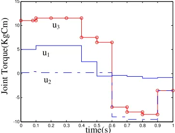
Figure 5. Control variable diagram based on EPSQP algorithm.
0 0.1 0.2 0.3 0.4 0.5 0.6 0.7 0.8 0.9 1 -10
-5 0 5 10 15
time(s)
Joi
n
t
T
or
q
u
e(K
gC
m
)
u1
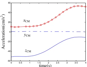
Figure 6. Diagram for barycenter acceleration of humanoid robot.
Summary
To reduce the damages against humanoid robot caused by falling and impact, firstly, establish a general dynamics model for humanoid robot, further analyze the characteristics of falling motion and establish a simplified, multilevel and inverted pendulum model for falling motion; secondly, adopt the optimum control method and convert the falling motion control problem of humanoid robot to the nonlinear control system problem that contains inequation constraint; finally, aiming at the defects of classic and minimal principle and classic SQP algorithm in optimizing effect, time and convergence rate, introduce an enhancing parameter optimization technique to conduct optimal control for the falling process of humanoid robot, and adopt configuration state set screening and EPSQP solution methods to improve the optimal control. The computer simulation shows that the improved parameter optimization method (EPSQP) can minimize the angular momentum during the falling of humanoid robot, each joint track change is smooth, barycenter acceleration is mild, optimizing time is relative short and the optimization effect is good.
Acknowledgement
This work was supported in part by a grant from Harbin Institute of Technology Robotics and System National Key Laboratory (SKLRS-2012-MS-06), Shenzhen Science and Technology Program (JC201006020820A and JCYJ20120615101640639), Team of Scientific and Technological Innovation of Shenzhen Institute of Information Technology (CXTD2-002), Natural Science Foundation of Guangdong Province, China (S2013010013779 and S2011040000672), Guangdong Vocational Education Information Technology Fund (XXJS-2013-1019), Scientific research and Cultivation Project of Shenzhen Institute of Information Technology (JS201704), Shenzhen Science and Technology Projection (JCYJ20160608151239996), Shenzhen Science and Technology Program (JCYJ20170306095849825).
Reference
[1] Masato H, Kenichi O. Honda humanoid robots development [J]. Philosophical Transactions of the Royal Socity.2007, 365(1850):11-19.
[2] Nishiwaki K, Kuffner J, Kagami S, et al. The experimental humanoid robot H7: a research platform for autonomous behavior. Philosophical Transactions of the Royal Society [J].Physical and Engineering Sciences, 2007, 365 (1850):79-107.
[3] Ke Wende. Research on Key Technologies of Motion Planning for Humanoid Robot Based on Similarity Locomotion of Human Actor [D].Harbin: Harbin Institute of Technology, 2013: 12-27.
0 0.5 1 1.5 2 2.5 3 3.5 4
-60 -40 -20 0 20 40 60
time(s)
A
cc
el
era
ti
o
n
(c
m
/s
2 )
xCM
yCM
[4] Eiichi Y, Igor B, Claudia E, et al. Humanoid Motion Planning for Dynamic Tasks[C]//IEEE-RAS International Conference on Humanoid Robots,2005:1-6.
[5] Kuffner J, Nakamura K, Kagami S, et al. Motion Planning for Humanoid Robots[C]//Proceedings of 11th International Symposium of Robotics Research,2003:1-11.
[6] Mitsuharu M, Kenji K, Fumio K, et al. Motion Planning of Emergency Stop for Humanoid Robot by State Space Approach[C]//IEEE/RSJ International Conference on Intelligent Robots and Systems,2007:2986-2992.
[7] Eiichi Y, Mathieu P, Jean-Paul L, et al. Whole-Body Motion Planning for Pivoting Based Manipulation by Humanoids[C]//IEEE International Conference on Robotics and Automation, Pasadena. 2008:3181-3187.
[8] Fumio K, Kiyoshi F, Hirohisa H,et al. Getting up Motion Planning using Mahalanobis Distance[C]//IEEE International Conference on Robotics and Automation, 2007:2540-2546.
[9] Zhong Q B, Hong B R, Pan Q S. Complex motion planning for humanoid robot based on embedded vision system[J]. Journal of Harbin Institute of Technology, 2010, 17(Supp1.2), 5-9.
[10] Zhang Tong. Research on Walking Control and Path Planning of a Humanoid Robot [D].Guangzhou: South China University of Technology, 2010:22-23.
[11] Zhong QiuBo. Research on Key Technologies of Motion Planning for Humanoid Robot [D].Harbin: Harbin Institute of Technology, 2011: 12-20.
[12] Lengagne S, Ramdani N. Safe motion planning computation for databasing balanced movement of humanoid robots[C]//IEEE International Conference on Robotics and Automation.2009:1669-74.
[13] Kiyoshi F, Shuuji K, Kensuke H, et al. An Optimal Planning of Falling Motions of a Humanoid Robot[C]//IEEE/RSJ International Conference on Inteligent Robots and Systems, 2007: 456-463.
[14] Bram Vanderborght, Björn Verrelst, Ronald Van Ham,et al. Objective locomotion parameters based inverted pendulum trajectory generator [J]. Robotics and Autonomous Systems, 2008, 56:738-750.
[15] Kajita Shuuji. Humanoid robots [M]. Guan Yisheng, Walls. Beijing: Tsinghua Univenity Press, 2007.
[16] Morawski J M. A Simple Model of Step Control in Bipedal Locomotion [J]. IEEE Transactions on Biomedical Engineering, 1978:544-560.
[17] Mousavi P N, Bagheri A. Mathematical Simulation of a seven link biped robot on various surfaces and ZMP considerations[J]. Applied Mathematical Modelling, 2007: 18-37.
[18] Miura H S. Dynamic Walking of a Biped Locomotion [J]. The International Journal of Robotics Research, 1984:60-74.
[19] Huang Q. Planning Walking Patterns for A Biped Robot [J]. IEEE Transaction on Robotics and Automation, 2001, 17(3):280-289.
[20] Hu L Y, Zhou C J, Sun Z Q. Biped gait optimization using spline function based probability model[C]//IEEE International Conference on Robotics and Automation, Orlando,FL,2006:830-835.
[21] Wang Qiang, Ji Junhong, Qiang Wenyi, Fu Peichen. Study on Biped Robot Control Based on Adaptive Fuzzy Logic and Neural Network[J].Chinese High Technology Letters, 2001, 11(7):76-78.
[23] Ke Xian xin, Gong Zhen bang, Wu Jia qi. Gait Optimization Based on Genetic Algorithm for a Biped Robot Climbing Upstairs [J].Journal of Applied Sciences, 2002, 20(4):341-345.
[24] Salatian A W, Yi K Y, Zheng Y F. Reinforcement learning for biped robot to climb sloping surface[J]. Journal of Robot, 1997, 14(4):283-296.
[25] Pandu R V, Sahu S K, Pratihar DK. On-line dynamically balanced ascending and descending gaits of a biped robot using soft computing[J]. International Journal of Humanoid Robot, 2007: 4(4):777-814.
[26] Teo K L, Jennings L S, Lee H W, et al. The control parameterization enhancing transform for constrained optimal control problems [J]. Journal of Australia Mathethatic Society, 1999, 40 (14): 314- 335.
[27] Zhong Qiubo, Pan Qishu, Hong Bingrong, Piao Songhao. Falling motion control of humanoid robot based on parametric optimum [J]. Robot, 2009, 31 (6): 594- 599. (in Chinese)
[28] Zhang Qi. Research on SQP Algorithm Under Nonlinear Optimization [D]. Qingdao: Qingdao University, 2008. 22- 28.
[29]Liu X L, Duan G R, Teo K L. Optimal soft landing control for moon lander [J]. Automatica, 2008, 44 ( 4) : 1097- 1103.
[30] Guan Y S, Neo E S, Kazuhito Y, et al. Stepping over obstacles with humanoid robots [J]. IEEE Transaction on Robotics, 2006, 22 (5): 958- 974.
[31] Fletcher R, Leyffer S, Toint P L. On the global convergence of a trust region SQP- filter algorithm [J]. SLAM Jo urnal on Optimization, 2002, 13 (3): 44- 59.
[32] Ke Wen-De, Cui Gang, Hong Bing-Rong, Cai Ze-Su, Yuan Quan-De. On biped walking of humanoid robot based on movement similarity. Robot, 2010, 32(6): 766-772
[33] Takano W, Yamane K, Nakamura Y. Capture database through symbolization, recognition and generation of motion patterns. In: Proceedings of the IEEE International Conference on Robotics and Automation. Roma, Italy: IEEE, 2007. 3092-3097