Ridge Basis Functions Collocation Method for Soil Water Movement Equations Under Infiltration with Two Point source Emitters

2018 International Conference on Modeling, Simulation and Optimization (MSO 2018) ISBN: 978-1-60595-542-1

Ridge Basis Functions Collocation Method for Soil Water Movement

Equations Under Infiltration with Two Point-source Emitters

Xing WANG

*

_{and Xin YANG}

Department of Applied Mathematics, Xi’an University of Technology, Xi’an, 710048, China

Keywords: Meshfree method, Soil moisture movement, Ridge basis function, Collocation method, Numerical simulation.

Abstract. Numerical simulation is an important method to research the soil y water infiltration under two point-source emitters. In order to improve the simulation precision and the practicability of numerical solution, a meshfree method based on ridge basis functions collocation method (RBFCM) is developed for solving 2D water movement equations in unsaturated soil under infiltration. The ridge basis functions are used as approximating functions to construct the method for the numerical solution of the water movement equations. The iterative method is used in solving the nonlinear matrix equation derived from water movement equations based on RBFCM. Compared with the traditional finite difference method and finite element method, the new method reduces the calculation time and calculation error. The numerical results of realistic water movement in unsaturated soil under infiltration meet the demands of actual problems well.

Introduction

Soil water movement is the most important part of the terrestrial water cycle and the recycling of pedosphere material. The mathematical models of the water flow in soils are mostly nonlinear partial differential equations whose analytical solutions are generally difficult to get in normal circumstances. Thus, a numerical method is currently the most effective way to solve soil water flow problems. In 2009, Guo and Sun [1] used the finite element method to solve the 2D soil moisture movement mathematical model, which included root water uptake under rainfall; it worked for some real-world situations. At the same time, Wang Zengtao[2] used the alternating implicit scheme method to solve the mathematical model of soil moisture movement under evaporation; the computational results were a good fit for the experimental results. In 2011, Li Huanrong and Luo Zhendong[3] used the finite volume element method to develop a two-dimensional unsaturated soil water flow equation, which is reliable, stable and practical.

The meshfree method has been developed over recent years. This type of method discrete the region of PDEs without the use of grid [4]. The initial idea for meshfree methods dates back to the smooth particle hydrodynamics (SPH) method for modeling strophysical phenomena [5]. In 1992, Nayroles et al. introduced the Diffuse Element Method (DEM) [6]; in 1994, Belytschko et al. improved the DEM and introduced the Element Free Galerkin Method (EFG) [7]. Since then, there has been a great deal of research into meshless methods. The Finite Point Method (FPM) introduced by Onate et al. [8], which is based on the Moving Least-Squares and the collocation method, is a truly meshless method. In particular, in 1990, Kansa introduced the radial basis function (RBF) collocation method for solving elliptic, hyperbolic and parabolic PDEs [9]. Later, the RBF was further developed by Schaback [10]. Hon et al. applied the RBF to the numerical computation of variable normal equations, the nonlinear Burgers equation and the Shallow water wave equation [11]. In 1999, Rippa carried out work on selecting the correct shape parameter c for the RBFs [12]. In 2003, Platte and Driscoll showed how the global RBF collocation method could be adapted to compute the eigenmodes of elliptic operators [13]. Therefore, the collocation-based meshless method has been an important meshless method in the current literature [14].

PDEs through radial basis function interpolation has yielded a number of significant results. In 2002, Gordon et al. examined the best approximation of some function classes using a manifold Mn consisting of sums of n arbitrary ridge functions [15]. Zhang [16, 17] studied the solvability of the interpolation with a ridge function in R2 and estimated the interpolation errors; moreover, he also gave an approximation for the limits of a linear combined ridge basis function for plane waves. Ismailov investigated the approximation of a continuous multivariate function f(x) = f(x1, . . . ,xd) by using the sums of two ridge functions in the uniform norm [18], proposed an explicit formula for the best L2 approximation for a multivariate function by linear combinations of ridge functions over some sets in Rn [19] and found a geometric method of deciding which continuous multivariate functions can be represented by sums of two continuous ridge functions [20]. Konovalov obtained estimates for the order of best approximation using polynomials and ridge functions in the spaces Lq

of classes of s-monotone radial functions which belong to the space Lp [21]. Shu presented a

meshless method, based on the weighted least-square method and ridge basis function interpolation (WLSR); the results of numerical examples applied to elastostatics are encouraging [44].

So far, the radial basis function collocation method (RBFCM) has yielded many important results in finding the numerical solutions to differential equations. However, studies of the theory of the ridge basis function collocation method and the practical applications of the numerical results are rare. The mathematical models of soil water movement are usually nonlinear convection-dominant diffusion equations.Several methods have been used to find their numerical solutions, such as the finite element method, the finite difference method, the finite element modified method of characteristics and so on. Nevertheless, improvements such as eliminating numerical oscillations and improving efficiency are still being studied.

In this paper, a new meshfree method based on RBFCM is proposed, which gives the numerical solutions of two-dimensional water movement in unsaturated soil. The existence and uniqueness of the solution to the proposed method is proved. Numerical examples show that the RBFCM is reliable, stable and practical to use in solving 2D unsaturated soil water problems.

Preliminaries

In this section, the mathematical model of soil water movement is introduced.

Generally speaking, soil water movement is a three-dimensional problem. If we assume that the soil is a porous media of isotropic non-deformable sand, the model of soil water movement can be treated as an axisymmetrical two-dimensional problem.

The soil moisture movement equation with soil water as the dependent variable is:

z K z D z x D x

t 

    

   

    

   

  

 ( )

) ( )

(    

 ₍₁₎

where θ is the soil volumetric water content (cm3_∙cm-3_{), t is time (in days) and D(θ) and K(θ) are the}

diffusivity (cm2_∙d-1_{) and hydraulic conductivity (cm∙d}-1_{) of the unsaturated soil movement. In this}

paper, the initial condition is

0

( , , )x z t ( , ),x z t 0,( , )x z

    (2) The boundary condition is defined as:

  

 ( , )

) , ,

(x z t ₁ x z

 (3) where θ0 is the water content of the topsoil (cm3·cm-3) andθ1 is the initial moisture content of the soil profile (cm3_·cm-3_).

Main Results: RBFCM

Construction of RBFCM

When the solution domain Ω is discretized by n nodes xi (i=1,2,…,n), then (x) can be

approximated by linear combinations of the ridge function φ(xi) :





     m v n i i h 1 1 )) ( ( ) ( )

(x  x   a_v x-x_i

 ,_xRd

(4)

where n is the node number, i is an unknown coefficient, av is a fixed direction and m is the total

number of the direction on the disk. In conventional numerical calculations, the Gaussian function_(_ax)_exp(_c(_ax)2)_{, the Multi-Quadrics function (ax) (c}2 _(ax)2_{), the}

Markoff distribution function (ax)exp(cax) and so on, are selected as the ridge basis functions where c is a constant (c>0).

For equation (1), the derivative is approximated in the following way at _{t t} n

n j i n j i n j i n j i n j i z K z D z x D x t _, 1 , 1 , , 1 , ( ) ) ( ) (                                  (5)

Here, we denote the function ~(x) as an approximation of (x):









         m v N i i m v N i i b i 1 1 1 1 )) ( ( )) ( ( ) ( ~ )

(x  x   a_v x-I_i   a_v x-B_i

 (6)

Let









m v1

))

(

(

)

(

x

-

I



a

_v

x

-

I



, then the approximation of (x)can be written as follows:





   

 i Nb

i i N i i 1 1 ) ( ) ( ) ( ~ )

(x  x  x-Ii  x-Bi

 (7)

where x (x,z),Ii,Bi, Niis the number of the nodes in the region andNbis the

number of nodes on the border.

Here, ridge basis functions are used as approximating functions to construct the method for the numerical solution of (1). From (1), (3), (5) and (7), the discrete form is given by:

1

1 1

1

1

( ) ( ) ( ), 1, 2, ,

( ) ( ) ( ) ( ( )) ( ( )) ( ) ( ) ( ( )) i b i b N N

n n n

i i j b

i i

N

n n n

i i N n n i i j N d d d d

t D t D

dx dx dz dx

d d t D dx dx                                   _ _  _ _  _{   }            _{ }  











j i j i

j i j i

j i j j

j i

j i j

B - I B B B

I I I I

Ι I I I

I B

I B I ( ( )) ( )

( ) 1, 2, ,

n n i d d t D dz dx

f j N

          _{   }  _{   }  _{  }       _{ }   j i j j I B I I (8) where ( ( )) ( ) ( ) n

n n K

f t z        j j j I

I I (9)

Let

( ) ( )

( ) ( ) t d D( ( ))d t d D( ( ))d

dx dx dz dx

 

      _   _  _   _

   

X I X I

Then (8) can be expressed in the following matrix equation:

F A

 (11) where

(0) ( ) ( ) ( )

( ) (0) ( ) ( )

( ) ( ) (0) ( )

( ) ( ) ( ) (0)

m

m

m

m

   

   

   

   

 _{  } 

 

 

 

  

 

  

  

 

 

 

 _{  } 

 

 

Φ

 

     

 

 

     

 

b i

b b b i

b i

i i b i

1 N 1 1 1 N

N 1 N 1 N N

1 1 1 N 1 N

N 1 N N N 1

B B B I B I

B B B I B I

I B I B I I

I B I B I I

(12)



n



N n n n N n n

i b

A 1,2,, ,1,2,, (13)

1( ), 1( ), , 1( ), ( ), ( ), , ( )

n n n _fn _fn _fn

  

 

  1 2  Nb 1 2  Ni 

F B B B I I I (14)

Linearization Scheme for the Nonlinear System

The matrix equation (11) is a nonlinear system. Here, we consider the iterative method to solve it. First, we derive the initial values of 0 _{at the nodes xi (i=1, 2,…, n) using (2) and as the predicted} values for 1_{.The values for D(}0_{) and K(}0_{) can also be calculated.} 0_{, D(}0_{) and K(}0_{) are then} used in the matrices  and F. Thus, the vector A can be calculated from (11). Then the values of 1 at the nodes xi (i=1,2,…,n) are obtained using (7).

Second, we can calculate more precise values of  1_{. For t=t} 1_{, we use the iterative method to} solve the nonlinear matrix equation. We denote 1 _{as }1(1)_{, D(}1_{) and K(}1_{) as D(}1(1)_{) and K(} 1(1)_{) and call them the correction values. So, for t=t}n+1_{, let }n _{be the predicted values of }n+1 _{and let} D(n_{) and K(}n_{) be the predicted values of D(}n+1_{) and K(}n+1_{). These are written as }n+1(1)_{, D(}

n+1(1)_{) and K(}n+1(1)_).

Third, we obtain the second iterative valued  n+1(2) _{by using the correction values }n+1(1)_{, D(}

n+1(1)_{) and K(}n+1(1)_{) as the next predicted value to solve (7).}

Finally, the above steps are repeated until the difference between the two iterative values is less than the maximum permissible error, that is

1( ) 1( 1) 1( 1)

max

n p n p n p

  _



  

 

 _{ , (15)}

where p is the number of iterations and ε is the maximum permissible error. Then  n+1(p) _{can be} considered as the final correction values for n+1_.

Numerical Examples and Validation of the Model Numerical Examples

  

   

 

    

  

   

   

 

     

 

0 , ) , ( ,

) , , (

) , ( ,

) 0 , , (

0 , ) , ( )

, , ( )

(

1 0

2 2 2 2

t z

x f

t z x u

z x u

z x u

t z x t

z x f z

u x

u u D t u

(16)

Here, assume that D(u)=1, [0,1][0,1]and ( , , )u x y t tsin(x)sin(y)denotes the exact solution of this model. u0, f and f1 are determined by the exact solution. A Gaussian function

) ) ( exp( )

(_{ax  c ax} 2

 is selected as the ridge basis function. Take a_i cos_i ,

8 2 1 8

1) / , , , ,

(   

 i i

i 

 . The Error Estimate is based on L2 Norms. Using the spatial step h=1/10,

the time step Δt=0.01 and T=1.0, we can obtain the results as shown in Figures 1 and 2.

[image:5.612.145.473.240.365.2]

Figure 1. Numerical solution of RBFCM. Figure 2. The exact solution.

Now, we consider a time step oft=0.01, until T=1.0, with different spatial steps and different parameters c. The results of the RBFCM are shown in Table 1.

Table 1. The results of the RBFCM for linear problem.

Inserted nodes(N) Spatial step(h) Parameters (c ) Calculation time(s) Calculation errors

44 1/4

0.470 4.294719 2.3973e-04

0.489 4.554394 1.6719e-04

0.500 4.321665 3.3324e-04

55 1/5

1.820 7.703303 1.5267e-04

1.790 7.821468 5.6379e-05

1.730 7.027453 2.3758e-04

1010 1/10

9.800 19. 637251 9.3096e-04

10.00 19.902975 7.1477e-04

[image:5.612.92.523.436.566.2]

10.10 19.202783 9.2443e-04

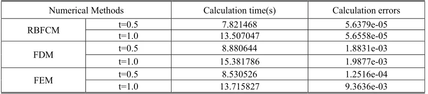
[image:5.612.93.521.614.708.2]

Table 2 shows the comparison of RBFCM with other methods such as the FDM and the FEM, where the time step is t=0.01, the spatial step h=1/10 and the nodes are 1010=100.

Table 2. Comparison of the results of the RBFCM with the FDM and the FEM.

Numerical Methods Calculation time(s) Calculation errors

RBFCM t=0.5 7.821468 5.6379e-05

t=1.0 13.507047 5.6558e-05

FDM t=0.5 8.880644 1.8831e-03

t=1.0 15.381786 1.9877e-03

FEM t=0.5 8.530526 1.2516e-04

Model Validation and Application

Here, the RBFCM is applied to find the numerical solution to a simulation of realistic water movement in unsaturated soil under evaporation. The Van Genuchten model is used to fit the soil water characteristic curve (h) and soil unsaturated conductivityK(h):

( ) / ( ) , 0,

( )

, 0,

n m r s r

s

l h h

h

h

   





    

  



 (17)



_1/



2

) 1

( 1 )

( m m

e l

e

sS S

K h

K    (18) where S_e (_r)/(_s _r),m11/n(n1), s is the saturated soil moisture content, _r is

the residual soil water content, Ks is the soil saturated hydraulic conductivity and n, m and  are

empirical parameters.

Table 3. Hydrodynamic parameters of experimental soil.

parameters r / (cm3cm3) s /(cm3cm3) / cm-1 n Ks / (cmmin-1)

value 0.15 0.38 0.02574 1.46 3.848

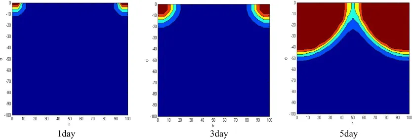
For the simulated land, the depth and the horizontal distance are all 100cm. The model simulated six days (d) with a time step of one day. The vertical direction and the horizontal direction of the soil were divided into 5 units and the spatial step was 20cm. According to the meteorological data for the region being simulated, from April 25 to May 15 2010, the average potential transpiration rate was calculated by ETO software to be 0.75cm/d.

The simulated water content distribution in the wetted soil after 1d, 3d, 5d and 6d are all shown in Figure 3.

[image:6.612.96.513.426.568.2]

1day 3day 5day Figure 3. Evolution of simulated water content distribution in wetted soil over time.

From the above figures, we can see that over time, the wetting front of the soil expands gradually. In other words, over time the soil water content increases. We can also see that the soil water content does not change a great deal and gradually approaches saturation near the drip irrigation source. The water content of the surface soil is sharp at a distance from the drip irrigation source. These results mirror the real-world situation.

Conclusions

reflects the movement of soil moisture more accurately than other methods, i.e., it is a good theoretical basis for further applications.

In addition, we found that the selection of the interpolation nodes, the ridge basis functions and the free parameter c, are all factors that influence the accuracy of the solution.

Acknowledgements

This work is supported by the National Natural Science Foundation of China (11626185) and Natural Science Basic Research Plan in Shaanxi Province of China (2017JQ1011).

References

[1] X. Guo, X. Sun, J. Ma . Numerical simulation for root zone soil moisture movement of apple orchard under rainfall-irrigation-evaporation [J]. Transactions of the Chinese Society for Agricultural Machinery, 40(11)(2009) 68-73.

[2] Z. Wang. Analysis and numerical simulation of soil moisture evaporation under the conditions of water storage simple pit irrigation [J]. Journal of Anhui Agricultural Sciences, 37(33)(2009) 164754-16478

[3] H. Li, Z. Luo. Self-discrete finite volume element simulation for two-dimension unsaturated soil water flow problem [J]. Mathematica Numerical Sinica, 33(1)(2011)57-68

[4] X. Zhang, K. Song, M. Lu. Research progress and application of meshless method [J]. Chinese Journal of Computational Mechanics, 20(6)(2003): 730- 742.

[5] L.B. Lucyt, A numerical approach to the testing of the fission hypothesis, The Astron. J. 82 (1977) 1013–1024.

[6] B. Nayroles, G. Touzot, P. Villon, Generalling the finite element method: diffuse approximation and diffuse elements, Comput. Mech. 10 (1992) 307–318.

[7] T. Belytschko, Y.Y. Lu, L. Gu, Element free Galerkin methods, Int. J. Num. Meth. Eng. 37 (1994) 229–256.

[8] E. Onate, S. Idelsohn, O.C. Zienkiewicz, R.L. Taylor, A finite point method in computational mechanics: applications to convective transport and fluid flow, Int. J. Num. Meth. Eng. 39 (1996) 3839–3866.

[9] E.J. Kansa, Multiquadrics-A scattered data approximation scheme with applications to computational fluid dynamics-I. Surface approximations and partial derivatives estimates, Comput. Math. Appl. 19 (8-9) (1990) 127–145.

[10] R. Schaback, Improved error bounds for scattered data interpolation by radial basis functions, Math. Comput. 68 (1999) 201–216.

[11] Y.C. Hon, K.F. Cheung, X.Z. Mao, E.J. Kansa, Multiquadric solution for shallow water equations, ASCE J. Hydraul. Eng. 125 (1999) 524–533.

[12] S. Rippa, An algorithm for selecting a good value for the parameter c in radial basis function interpolation, Adv. Comput. Math. 11 (1999) 193–210.

[13] R.B. Platte, T.A. Driscoll, Computing eigenmodes of elliptical operators using radial basis functions, Comput. Math. Appl. 48 (2004) 561–576.

[15] Y. Gordon, V. Maiorov, M. Meyer, S. Reisner, On the best approximation by ridge functions in the uniform norm, Constr. Approx. 18 (2001) 61–85.

[16] L. Zhang, Error estimates for interpolation with ridge basis function, J. Fudan Univ. (Nat. Sci.) 44 (2) (2005) 301–306.

[17] L. Zhang, Approximation to limited linear combined ridge basis function of plane wave, J. Shandong Univ. (Nat. Sci.) 41 (6) (2006) 87–92.

[18] Vugar E. Ismailov, Characterization of an extremal sum of ridge functions, J. Comput. Appl. Math. 205 (2007) 105–115.

[19] Vugar E. Ismailov, A note on the best L2 approximation by ridge functions, Appl. Math. E Notes 7 (2007) 71–76.

[20] Vugar E. Ismailov, Representation of multivariate functions by sums of ridge functions, J. Math. Anal. Appl. 331 (2007) 184–190.

[21] V.N. Konovalov, D. Leviatan, V.E. Maiorov, Approximation by polynomials and ridge functions of classes of s-monotone radial functions, J. Approx. Theory 152 (2008) 20–51.