BIROn - Birkbeck Institutional Research Online
Brummelhuis, Raymond and Luo, Zhongmin (2019) Bank net interest
margin forecasting and capital adequacy stress testing by machine learning
techniques. SSRN Journal , ISSN 1556-5068.
Downloaded from:
Usage Guidelines:
Please refer to usage guidelines at
or alternatively
Bank Net Interest Margin Forecasting and Capital Adequacy Stress
Testing by Machine Learning Techniques
Raymond Brummelhuis
∗Zhongmin Luo
†March 31, 2019
Abstract
The 2007-09 financial crisis revealed that the investors in the financial market were more concerned about thefutureas opposed to thecurrentcapital adequacies for banks. Stress testing promises to complement the regulatory capital adequacy regimes, which assess a bank’s current capital adequacy, with the ability to assess its future capital adequacy based on the projectedasset-lossesandincomesfrom the forecasting models from regulators and banks. The effectiveness of stress-test rests on its ability to inform the financial market, which depends on whether or not the market has confidence in the model-projected asset-losses and incomes for banks. Post-crisis studies found that the stress-test results are uninformative and receive insignificant market reactions; others question its validity on the grounds of the poor forecast accuracies using linear regression models which forecast the banking-industry incomes measured by AggregateNet
InterestMargin. Instead, our study focuses on NIM forecasting at an individual bank’s level and employs both linear regression and non-linear Machine Learning techniques. First, we present both the linear and non-linear Machine Learning regression techniques used in our study. Then, based on out-of-sample tests and literature-recommended forecasting techniques, we compare the NIM forecast accuracies by 162 models based on 11 different regression techniques, finding that some Machine Learning techniques as well as some linear ones can achieve significantly higher accuracies than the random-walk benchmark, which invalidates the grounds used by the literature to challenge the validity of stress-test.Last, our results from forecast accuracy comparisons are either consistent with or complement those from existing forecasting literature. We believe that the paper is the first systematic study on forecasting bank-specific NIM by Machine Learning Techniques; also, it is a first systematic study on forecast accuracy comparison including both linear and non-linear Machine Learning techniques using financial data for a critical real-world problem; it is a multi-step forecasting example involving iterative forecasting, rolling-origins, recalibration with forecast accuracy measure being scale-independent; robust regression proved to be beneficial for forecasting in presence of outliers. It concludes with policy suggestions and future research directions.
Keywords: Machine Learning; time series forecasting; forecast accuracy; bank capital; stress testing; net interest margin; systemic risk.
1
Introduction
The 2007-09 financial crisis revealed that the financial market was more concerned aboutfutureas opposed tocurrentcapital adequacy problem for large financial institutions, some of which failed or nearly failed but were judged to be ”well-capitalized” by the on-going regulatory capital criteria; see a list of such financial institutions in Schuermann (2014). Also, it was clear that such concerns about future capital adequacies with a few large banks (particularly, the so-called global systemically important banks or G-SIBs) can quickly transform into the collapses of financial and economic systems or into a systemic risk. Schuermann’s study found that the stress-test exercise conducted by the US regulators in May 2009 unprecedentedly disclosed important information about the projected capital and net revenue results under the worse-case-scenario for some of the largest banks, which, corroborated by observations from Krugman1, effectively regained
∗
Dept. of Mathematics & Computer Science, Univ. of Reims, Reims, France, [email protected] †
Dept. of Economics, Mathematics & Statistics, Birkbeck, Univ. of London, England, [email protected].
1Krugman P., 14/07/14, ”the stress tests marked the end of the financial panic during the financial crisis; after stress testing, the three
investors’ confidence in the banking industry so that the banks were able to raise needed capitals from less volatile markets, and effectively end the crisis. Also, the study by Schuermann highlighted that, whilst proper stress test requires modelling three components for the banks, namely,asset losses,net revenuesand
balance sheet dynamics, regulators, banks and researchers have focused mainly on quantifying the asset losses when assessing banks’ capital adequacy and that the literature about the latter two is very limited. In this study, we focus on forecasting the second component. Meanwhile, we reserve the third component of stress testing for future research; see for example Hirtleet al(2015), which included current practice of assuming constant asset growth rates estimated from historical data.
Stress testing has become a central tool used by global regulators to manage financial stability with the promise to address investors’ real concerns about banks’ future capital adequacies manifested during the financial crisis. Typically, national regulators use their own stress-test models developed for a representative bank based on data collected about banks and macroeconomic variables to project the future capital needs for a typical bank under a set of forward-looking severely stressed macroeconomic scenarios and baseline (normal) macroeconomic scenarios (see for example Hirtleet alfor the US). Then they use the results to evaluate the numbers reported by individual banks, which include individual banks’ future asset-losses, incomes and future capital plans, projected by the banks’ own forecast models under the set of forward-looking economic scenarios; based on the evaluation results, regulators identify those banks which need to replenish their capitals and release such results to the public. However, a recent study by Kupiec (2018), which forecast total incomes (interest incomes plus non-interest incomes) for a representative bank based on regulator-like models, raised serious concerns about the absence of information about how regulators evaluate banks’ forecasted numbers and concerns about data overfitting and lack of out-of-sample tests about the forecast accuracies of the stress-test models.
Clearly, the creditability of the stress testing as a regulatory tool for financial stability is founded on its ability to inform the financial market, which, in turn, depends on its ability to establish or maintain the market’s confidence in the results projected by the three forecast modelling components, namely, the respective models used by regulators and banks to project banks’ future asset-losses, incomes and balance sheet dynamics. However, some of post-crisis literature is very critical about the stress testing. For example, Glasserman and Tangirala (2015) highlighted that the US stress-test results have become predictable and uninformative year after year, and therefore subject to gaming by banks. Some others criticized the soundness of first two modelling components of stress-test. For example, Acharya, Engel and Pierret (2014) criticized that the risk weights used to project banks’ asset-losses are not risk-sensitive. Using linear regression models, two post-crisis papers respectively by Guerrieri and Welch (2012) and by Bolotnyy, Edge and Guerrieri (2015) found that the forecasted industry-wide Aggregated NIM, which is defined as, at the banking industry level, the net interest earnings to interest-earning asset ratio, is mostly not as accurate as those forecasted by a simple Random-walk model. Thus, the authors of both papers questioned the credibility of the stress test, which we refer to as thePredictability or Forecast Accuracy Problem for Aggregate NIM. All above literature has taken a top-down approach to study the forecast accuracy of NIM models for either a representative bank level (see Hirtle et al’s or Kupiec’s) or for Aggregate NIM at the banking-industry level (see the above two Aggregate NIM literature); unfortunately, no post-crisis literature available in public domain has adopted a bottom-up approach to examine whether the forecast accuracy problem with Aggregate NIM also exist for the bank-specific NIM forecast model used to predict future NIM for a specific bank (to which we refer as a Bank-specific model); in this study, we take up the challenge.
We next turn to explain why we have chosen to study NIM as the net income metric for banks rather than other metrics such as total income (like Kupiec’s) or Return on equity (ROE) or Return on asset (ROA).
First, non-interest incomes for banks such as the capital gains from trading, advisory fees, as a percentage of banks’ total incomes (which also include interests earned from interest-earning assets such as loans, bonds, etc.) have decreased sharply after the financial crisis according to our study based on data from the US Fed2) across the Euro Area, the United States and the world as a whole. The sharp decrease coincides with a period of post-crisis regulatory reforms which have led to increased capital requirements for investment-banking businesses so that banks have moved back to traditional interest-earning businesses such as lending instead of mainly non-interest-earning businesses such as trading. Thus, NIM has become more reflective of banks’
main business activities than before.
Also, according to a ECB’s study (2010), the ROE (return on equity) was criticised after the financial crisis for its short-term focus and incentivizing banks for increased risk-taking while neglecting long-term profitability; the ROA (return on asset) tends to be flat across time, containing little information for predicting potential future profit falls.
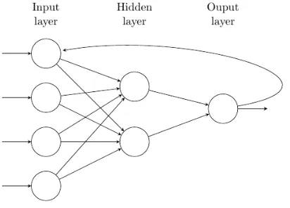
In our study, we will examine whether theforecast accuracyproblem for Aggregate NIM raised in the above NIM literature exists for Bank-specific NIM. The forecasting models we will use include both the linear models used in NIM literature and Non-linear regression models from the Machine Learning arena such as the Regression Tree and its Ensemble-version, Gaussian Process Regression, Support Vector Machines and the NARX (or Nonlinear AutoRegressive models with eXogeneous inputs) version of Recurrent Neural Networks (or RNN, see Linet al(1996) for an introduction of NARX version of RNN and see Graves (2014) for a recent introduction for RNN) and which, from a statistician’s viewpoint, can be considered as non-linear regression models.
In the remainder of this introductory section, first, we will discuss the relationships between capital adequacy, bank income and stress test; then we will present the essence of bank-specific NIM forecasting by Machine Learning Techniques, including the economic principles followed by our feature selections; finally, we will survey recent literature on NIM study, review some forecasting techniques from the literature, then present a summary of the research gaps which motivated this study and a summary of what we believe to be this paper’s main contributions.
1.1
Capital Adequacy, Bank Incomes and Stress Test
As indicated in the FCIC report (the US Financial Crisis Investigation Commission), the global financial crisis was caused by a panic about the financial system triggered by the collapses of a few G-SIBs3, which in its turn resulted from the fear on the part of the creditors and business partners that these G-SIBs might not be able to honourfuturefinancial obligations, leading creditors and investors to refuse to roll over the existing short-term funding to these G-SIBs such as 90-day Asset-backed Commercial Paper4. Thus, our study will focus on the G-SIBs.
According to Basle III’s capital adequacy requirements (2010), a bank’s accounting capitalKA
t should, at a reference datet, exceed a fixed constantktimes the risk-weighted value of its assets orRWAtat timet:
KtA≥k·RWAt, (1)
wherekis the so-calledcapital adequacy ratio. The bank’s accounting capital is, by definition, the sum of itsequity E1
t (contributed by its shareholders and subject to a bank’s own capital planning, e.g., new share issuance and share buyback.), and itsretained earnings E2
t, which is the income generated from its business and investment activities minus the dividends paid to its shareholders.
The objective of stress testing is to examine whether or not at some reference datet, (1) still holds at future timest+h(h:=1,2,· · ·,H), given a set of exogenously given economic scenarios denoted byωt+hrelated to
timet+h, which represent normal and or severely adverse future economic conditions contemporaneous with a response variableyt+h|tfor which we will take the predicted NIM att+h, given information available att; symbolically,
KAt+h|t(yt+h|t, ωt+h)≥k·RWAt+h|t(ωt+h) (2)
whereKA
t+h|t(yt+h|t, ωt+h) denotesh-step ahead projected accounting capital for timet+has a function of both
h-step ahead NIM to be forecasted (denoted by yt+h|t) andωt+has well as other information at timet, and similarly for the right hand side.
The 2007-09 crisis manifested the significant difference between (1) and (2) in that the former is concerned with banks’ current capital adequacy, whereas, the latter is with their future capital adequacy. During the crisis, the fear of future failure severely affected the share prices of banks such as Morgan Stanley, which lost
3Our study includes 6 US G-SIBs:https://bit.ly/2xC8wh1
almost 30% of its share values on the day after the Lehman debacle despite the fact that Morgan Stanley had $181 billion in cash, just posted earning results that defied analysts’ expectations and had a healthy capital ratio5. This indicates that the real concerns of investors and banks’ creditors were about their future as opposed to their current capital adequacy. The purpose of stress testing and that of this study is to address such real concerns.
Reliable stress-test rests on finding good models for the two sides of (2). A lot of research efforts (see for example McNeil, Frey and Embrechts, 2015) has gone into the modelling side ofRWAt+h|t(ωt+h), and in particular of the valuation of the different assets which constitute the bank’s portfolio. As regards the portfolio itself, quantitative models for banks’ balance sheet dynamics are unrealistically simple in practice; see examples of assuming constant growth rate for assets in Hirtleet al’sand Kupiec’s. Modelling balance sheet dynamics is an interesting and challenging topic6: the future equity depends on strategic decisions such as share buyback or new share issuances, which will depend on future capital projection and make predicting future equity holdings a ”nested forecasting problem”. Modelling the balance sheet dynamic is outside of the scope of the present paper. In this paper we will concentrate on the left-hand side of (2), and in particular onforecasting retained earningscomponent.
1.2
Essence of Bank-specific NIM forecast by ML-techniques
Given a set of exogenous economic scenarios contemporaneous with timet+h and conditional on other information at timet, the goal of this study is to forecasth-step ahead NIM, which will then be used to check whether or not the capital adequacy condition (2) holds for a specific bank on on-going basis in stress testing. To that end, as indicated in section 2, we include classical statistical and more recent Machine Learning regression techniques in our study. We will refer to both of these below as Machine Learning Regression Techniquesor simply asML-Regression Algorithms. In contrast with the Classification models used in Brummelhuis and Luo (2019a), which are used to predictdiscrete variables, the aim of Machine Learning Regression is to devise computerised algorithms which predict the value of one or morecontinuous response variables, on the basis of a vector-valued feature variable with values in some finite dimensional vector spaceRd. Since our forecast models involve non-linear Machine Learning techniques, these inevitably
contain elements of parameterization choices, see Brummelhuis and Luo (2019b) for a reference in the context of classification. We refer to Hastie, Tibshirani and Friedman (2008) for an overview of modern Machine Learning and Tashman (2000) for a comprehensive review of multi-step forecasting including some forecasting techniques used in this study. In this study, we also compare the forecast accuracy of our regression models with those of a benchmark model; see Brummelhuis and Luo (2019b) for a benchmarking exercise in the context of classification. At the beginning of forecasting, it is important to determine whether to formulate a problem as a classification or a regression one and a wrong decision at this point can lead to nonsensical results; see an example of potential nonsensical probabilities among other implications as a result of using cross-sectional regression as opposed to classification for constructing CDS proxy rates in Brummelhuis and Luo (2018c).
Denoting NIM at time t byyt, we can express the models used for this study schematically:
yt+h= f(yt+h−1,Xt+h, θh)+t+h, (3)
Whereyt+h−1denotes an AR(1) term for NIM which we introduce for reasons discussed below.Xtis the vector of exogenous feature variables representing the macroeconomic variables or bank-specific microeconomic variables (see a list of feature variables in Appendix A.1), both contemporaneous withyt+h; f is a function
depending on a set of parameters denoted byh-specificθhandt+his the forecast error term measured as the gap betweenydt+hforecastedex-anteandyt+hobservedex-post.
Equation (3) applies to both training and forecasting: during training, h =0, we train equation (3) on training samples; during forecasting,h > 0, we can form forecasts based on the learned functional form with parametersθbh.
5Wharton;https://whr.tn/2St2kiF
6Balance sheet modelling requires granular predictive models, e.g., product-specific account balance origination, roll-over rates,
During the training stage, we need to make a few related modelling choices: (1) whether we want to forecast based on a fixed forecasting origin or rolling origins; (2) if the choice of rolling origins is decided, whether we want to just update our training set with new data or we want to recalibrate our models at each roll of forecasting origin before forecasting; (3) whether we want a certain feature variables always included in our final model or not for practical reasons, e.g., the board of a company or the regulator might want to see the response of NIM with regard to CPI index, etc. First, fixed-origin forecasting only produces a horizon-specific forecast and a horizon-specific forecasting error, which makes its results susceptible to data noise and makes it difficult to judge the forecast accuracy; in contrast, rolling-origin forecasting leads to multiple horizon-specific forecasting errors, which permits one to estimate a distribution of forecasting errors. Hence, we choose rolling-origin forecasting as recommended by Tashman in our study. Second, given that both our forecasting object and most of our feature data are quarterly, we recalibrate our model to a rolling training set to allow our models to pick up the potential signals in data between quarters. Third, our feature selection is mainly driven by economic principles, we choose to include a default set of economically motivated feature variables, which we call standard feature selections (see FS1-FS10 in Appendix A).
As a result, we evaluate forecast accuracy based on a series of horizon h-specific forecasting errors defined as bh = yt+h− dyt+h, which are always out-of-sample in that sense that the observed yt+h is not
part of the training sample that ends at forecast origint. Bergmeir and Hyndman (2018) is a recent study which includes a discussion of such practice in the context of Leave-one-out cross validation (LOOCV) as a special case ofK-fold cross validation. As discussed further in section 2.2, from each rolling window, we obtainh-specific out-of-samplet+h; we collectt+hfrom all rolling-origin forecasts to arrive at a statistics for forecast accuracies measured by a metrics such as Root-mean-squared-forecast-error or RMSE; see section 2.11 for further details regarding the choice of forecast accuracy metrics.
In the remainder of this section we explain the rationale underlying the 10 different Standard Feature Variable selections as described in Appendix A.1, which are economically motivated; we use these 10 Feature Selections in all models with the exceptions of Principal Component Regression and Stepwise Regression, which, for reasons explained in section 2, are based on their own Feature Selections shown in Appendix A.3 and Appendix??respectively. In the same vein, the study by Busch and Memmel (2014) contains a discussion about determinants of NIM.
1. First of all, banks are paid for providing two related financial intermediary services,Term Transformation
(TTS) andInterest Rate Risk Management(IRM). Traditionally, banks generate interest incomes by paying their depositors the low rates on the short end of the interest rate curve in exchange for deposits (which are short-term on average) while earning the high rates on the long end of the curve from activities such as mortgage lending. As a result, customers can transform their asset-maturity profile, for example, from short-term cash into long-term houses, which is called Term Transformation. Meanwhile, to provide such intermediary services, banks have to invest in managing interest rate risk, for example by hedging interest-rates using derivatives such as interest rate swaps and swaptions for risks related to interest rate level and volatility respectively. Clearly, both TTS and IRM are influenced by interest rate level and interest rate volatility. However, empirical experience from experimenting with the so-called ”Merrill Lynch Option Volatility Index” or MOVE, which is a the standard index for tracking implied interest rate volatility, suggests that interest rate level movements are more important for the bank-specific NIM models of our study. Meanwhile, for loans of revolving exposures such as revolving lines of credits, as expected, our experiences show that MOVE contributes significantly to explain the variations of NIM at asset class level, which is out of the scope of this study. In our study, we therefore naturally use theSlope of the Interest Rate Curve, defined as the gap between 10-year and 3-month treasury yields, as one of our feature variables; see Covas, Rump and Zakrajsek (2014) as an example of such a practice in the NIM literature, and Appendix A for further details.
link thiscollective credit riskto two broad equity market indices, the S&P 500 and the VIX, the implied volatility index for equity options, which we use as feature variables. In addition, we have included a bond spread index, which is also indicative of Credit Risk: see Appendix A for details.
3. Thirdly, empirically, the NIM shows a certain persistence, which can be explained by the fact that banks often have large volumes of fixed-rate loans. Furthermore, banks’ operational costs such as staff, properties and equipment are relatively stable between two consecutive reporting periods and the efficiency of a bank’s management team and its market position, as indicated by metrics such as the banks’ own credit standing, are relatively stable. Our feature selection needs to reflect this persistence of bank incomes, and we have done so by including a 1-period lagged Autoregressive term of NIM as a feature, for which Appendix B.2 provides a justification in the context of linear models, by examining the autocorrelations. We recognize that for the non-linear models such an argument is not conclusive and that, ultimately, the question of how many lags have to be included can only be answered empirically, for each algorithm separately. We note that basically all post-crisis NIM literature only use AR(1), without further justification7.
1.3
Literature, Research Gaps and Contributions
NIM and Forecasting Literature
Based on their forecast objectives, the NIM literature can be divided into papers focused on forecasting NIM for a specific bank using bank-specific NIM models and those on forecasting NIM at banking-industry level using Aggregate NIM models. In this section, we review the techniques used by both types of literature so that we can include them in our study of Bank-specific NIM forecasting.
The paper by Ho and Saunders (1981) is the first studying Bank-specific NIM using classic Multiple Linear Regression techniques, including both cross sectional and time series regression, to try and understand the determining factors of a bank’s NIM, by linking this NIM to a number of microeconomic and macroeconomic variables.
As for Aggregate NIM, Grover and McCracken (2014) find support for its predictability, using Factor-based NIM models via Principal Component Regression. Another Aggregate NIM study is the one of Covas, Rump and Zakrajsek (2014), who present a Fixed-Effect Quantile Autoregressive Regression (FE-QAR) model which significantly outperforms its Fixed-Effect Linear counterpart. Contrary to other papers on NIM, they investigate a non-linear model by forecasting the conditional density for NIM instead of the conditional mean as done in linear forecast models, but their study differs from ours in following respects: first, the modelling object is the NIM for a representative or ”average” bank (which is still aggregate NIM) and the approach taken is a top-down approach by assuming the same set of feature variables across banks to forecast the NIM for a representative bank while, in this study, we take bottom-up approach to forecast the NIM for a specific bank, which allows for bank-specific feature selections and potentially leads to more accurate forecasting; second, they use the Linear Fixed Effect model as the benchmark (against which forecasting performance of other models has to be tested) while we will use the Random Walk, the same benchmark-model shared by most of the literature including two important NIM studies on Aggregate NIM to be discussed next. Similar to the above authors, Kupiec’s study focused on forecasting a representative bank’s total income calculated as the average total income across all banks in sample; in that sense, it is a top-down Aggregate NIM study. We note that, Kupiec’s is the only study on bank-income forecast which includes a Machine Learning technique, specifically, the so-called least absolute shrinkage and selection or Lasso for its feature variable selection (see Hastie, Tibshirani and Friedman), which, however, is a technique for variable selection rather than a forecasting technique; in addition, the target variable in Kupiec’s is bank’s total income rather than Bank-specific NIM, on which we choose to focus for reasons discussed above.
We next turn to the two post-crisis Aggregate NIM studies of Guerrieri and Welch (2012) and Bolotnyy, Edge and Guerrieri (2015). Using RMSE as the forecast accuracy metric, both papers found that the forecast accuracies of their Linear Regression models, which included an AR(1) term for NIM as one of its explanatory variables, were indistinguishable from those of the random-walk benchmark. As a result, both papers raised serious concerns about the relevance and effectiveness of stress tests, which we referred to
as thepredictability or forecast accuracy Problem for the Aggregate NIM. As regards feature variable selections, Bolotnyy, Edge and Guerrieri used only treasury-yield variables as features, whereas Guerrieri and Welch included a wide range of macroeconomic variables. We note in passing that interest-rate only variables may not be very useful in a flat-rate environment such as the one prevailing after the 2008-09 crisis. As regards the data samples, the main results from Bolotnyy, Edge and Guerrieri’s are based on data sample ranged from 1989Q4 until 2008Q3, and thus did not completely cover the financial crisis up till its end in 2009Q2, particularly, the post-crisis expansionary periods8, which prevents their results from being extrapolatable to forecasting NIM for post-crisis expansionary periods. Similarly, the Aggregate NIM study conducted by Guerrieri and Welch was based on data up to 2009Q4.
In contrast with the above two NIM studies, which used rolling-origin forecasting, Kupiec’s study, however, was based on fixed-origin forecasting; thus, the assessment of his forecast accuracy using RMSE was based on only 12 sample points for forecast errors while assuming constant forecast errors across forecasting horizons. The training set used in Kupiec’s study included data from March 1993 to June 2008, but excluded the Lehman’s default (15 September 2008), its ensuing periods and the post-crisis expansionary periods; its out-of-sample test was based on the 12 quarters following June-2008. In our view, the sample size seems to be small and rolling-origin forecasting is desirable.
Regarding multi-step forecasting techniques, Bolotnyy, Edge and Guerrieri found that theiterated multi-step approach outperforms thedirectmulti-step one. This is in line with other papers from the forecasting Literature such as Macellino, Stock and Watson (2005), who compared the forecast performances of it-erated multi-step and direct Multi-step forecasting using 170 different time series of US macroeconomic variable data, finding that the former outperforms the latter although the former is more vulnerable to misspecification errors.
Regarding the empirical comparisons of Machine Learning algorithms for forecasting purposes, we mention the paper by Ahmed, Gayar and El-Shishiny (2010), who found the following ranking in terms of forecast accuracy for the three algorithms studied in this paper: Neural Network, Gaussian Processes Regression and Support Vector Regression. We note however that their empirical study was restricted to Single-step forecasting only and was not related to banking.
We finally comment on the issue of forecast accuracy metrics. Based on the study of 90 annual and 191 quarterly economic time series data, Armstrong and Collopy (1992) found that the RMSE as performance criterion is not reliable for comparing forecasting performances for different time series of different scales. As an alternative, they propose to use the so-called Relative RMSE as a measure of forecasting errors. Hyndman and Koehler (1992) proposed Mean Absolute Squared Error (MASE) as a general measure for forecasting accuracy. A more recent study by Chen, Twycross and Garibaldi (2017) proposed an alternative error metric called the Unscaled Mean Bounded Relative Absolute Error orUMBRAE, and compared a long list of metrics including the above ones, finding from their empirical comparison study that UMBRAE is superior among a list of error measures for Time Series forecasting; see further discussion in section 2.
Research Gaps
Following the preceding literature survey, we identified the following research gaps which motivated our study in this paper:
1. Literature on stress-test have raised various concerns about the accuracies of the forecasting models for bank income used in these tests, and in particular about the accuracy of Aggregate NIM forecasts; however, despite the fact that the stated objective by regulators is to gain confidence of investors and creditors in the banks and financial system, no literature is available in public domain on the accuracies of NIM forecast models used by banks for stress-tests. Without such information, the regulators and banks may leave investors and creditors in doubt about stress-test results and even existing confidence in them could be diluted, which might explain the failure of some stress-test disclosures to receive significant market reactions as highlighted in some studies.
2. As regards the modelling techniques, existing NIM literature only use classical Linear Regression
8The US National Bureau of Economic Research shows that its economy resumes its expansion from June 2009, 1 month after the
techniques in their forecasting models although non-linear Machine Learning techniques can be used to construct time-series forecast models and might bring out new insights.
3. Empirically, NIM data are known to be non-Gaussian and heavy-tailed; the results from existing literature are typically based on Linear regression models, which are typically estimated by Ordinary Least Square methods; LS estimators are known to be vulnerable to outliers. Alternative regression techniques might bring new insights or even lead to different results to those from existing literature.
4. With regard to the data sampling, post-crisis bank-income studies cited above only covered part of the latest economic cycle without including the economically expansionary period after the financial crisis; since now we have a bigger data sample, increased forecasting accuracy based on out-of-sample test from bigger sample size is possible.
5. Using the RSME to compare the forecasting performances of different models applied to different banks with varying data scales can be problematic. Arguably, the use of scale-independent forecast accuracy measures such as the Rel-RMSE or the UMBRAE (see 2.11) is more appropriate for such situations and may lead to different conclusions.
6. As a time-series forecasting study, ours include non-linear Machine Learning techniques, which might bring out insights about time series forecasting performance comparison. Except for one study, which only examined Single-step prediction for non-financial data, existing empirical performance-comparison literature rarely include any models from the Machine Learning area. Such models may be serious competitors to the classical models (and we will indeed find this to be the case for at least one class of ML-models).
Contributions of the paper
The paper makes the following contributions to the existing literature:
1. It is the first systematic study on the forecast accuracy problem for Bank-specific NIM. As indicated in section 3, in contrast with the problem raised in the literature about Aggregate NIM, we find that Bank-specific NIM can be predicted with much better accuracy than does the random-walk benchmark by both linear and non-linear regression models, which suggests that Stress Test should not be discredited simply because of the forecast accuracy problem with Aggregate NIM.
2. We show that non-linear Machine Learning regression techniques achieve superior forecast accuracies, notably the NARX version of RNN (cf. section 2), followed by the Gaussian Process Regression (or GPR) and Support Vector Regression (or SVR); the rank-ordered forecast accuracies in our study as shown in Section 3 are in line with those reported in a separate study by Ahmed, Gayar and El-Shishiny (2010) as discussed in section 1.3; however, our studies are conducted in the context of banking data and of Multi-step forecasting.
3. Within Recurrent Neural Network, Bayesian Neural Network achieved the best performances out of different backpropgations, which is consistent with findings from the literature, such as Zhang, Patuwo and Hu (2003).
4. The study represents an application of Robust Regression in both Linear and Factor-based regression models; in presence of outliers in NIM data, Robust Regression is shown to significantly improve forecasting results, as indicated by the performance improvements in Section 3 shown by MLR vs ML, PCR-MLR vs PCR-ML.
5. The paper is an example of applying the following forecasting techniques: multi-step forecasting in-volving rolling origins, model recalibration, Leave-one-out cross validation for time series modelling, choice of forecast accuracy metrics between scale-dependent RMSE and scale-independent metrics such as UNMBRAE, RelRMSE, etc.
7. As for policy suggestions, we recommend that regulators take steps to disclose forecast accuracy information based on literature-recommended forecasting techniques such as out-of-sample tests, rolling-origin forecasting, model recalibration as well as non-linear Machine Learning techniques as part of the forecast models used by banks and regulators themselves, which should contribute to improve confidence on part of investors and creditors in financial markets and to maintain the financial stability. Furthermore, banks should be encouraged to conduct research into forecast models at more granular levels such as asset classes, which will help regulators and banks to identify the vulnerabilities in business areas in G-SIBs at build-up stages before they transform into a crisis.
The rest of the paper is organized as follows:
In section 2, we briefly review linear regression and Machine Learning regression techniques, which we have used to investigate potential forecast accuracy problem with Bank-specific NIM. Section 3 summarizes our empirical results; we do an inter-model comparison, and identify the best performing ones, which is followed by discussions about the empirical results for each model type separately and the conclusions which we believe can be drawn from this paper’s results. Three appendices, A, B and C, respectively list the precise feature selections, present data description and summary statistics for the NIM as well as a collection of the different figures and tables which form the basis of the discussion for model-specific results presented in section 3.
2
Regression models via ML-techniques
Classical statistics include a wide range of regression techniques for forecasting; in addition, modern Machine Learning arena also provides regression models that are based on Machine Learning techniques. In our study, we follow the literature (see Hastie, Tibshirani and Friedman, 2008) by referring to both as Machine Learning Techniques or simplyMachine Learning-regression algorithmsto include all regression models of distinct types; we reserveML modelfor representing Multiple Linear regression models only. As mentioned above, our objective is to forecast the multi-step ahead NIM values for a given bank in response to a set of exogenously given economic scenarios in the context of stress-test; thus, a multi-step time series forecast model as indicated by equation (3) needs to be constructed, trained before being used to forecast NIM. Given that a wide range of model choices and feature variable selections are available, we need to start with a Random Walk benchmark, which is a practice shared by two of the post-crisis NIM forecasting literature discussed above and advocated by forecasting literature in order to compare forecast accuracy amongst competing models based on out-of-sample tests; see a discussion by Hyndman9.
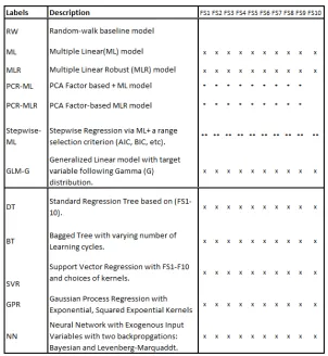
In this section, we will present a brief introduction for each of the Machine Learning-regression algo-rithms used in our investigation. Table 1 summarizes some of the Machine Learning-regression algoalgo-rithms that we have tested using a list of so-called standard feature variable selections abbreviated as FS1-FS10 (marked by an ”x”), for which detailed descriptions are available in Appendix A.1; in addition, we present a list of feature selections in Appendix A.2, which we investigated but found to achieve lower accuracies than the standard ones. Excluding the random-walk model (labelled as ”RW”), we tested a total of 162 models for predicting bank-specific NIM from 11 different Machine Learning-regression algorithms, including 108 models in Table 1 and additional 54 models in Table 5 in Appendix A.2. In addition to their individual sections below, Appendix A.3 and??contain more details about Principal Component Regression and Step-wise Multiple Linear Regression respectively. Regarding the types ofML-Regression algorithmsinvestigated in the study, we choose popular ML-Regression ones based on a survey of NIM literature (cf. Section 1.3), which is not meant to be exhaustive.
2.1
Random Walk: the benchmark model
We follow common practice and two prominent NIM forecasting literature (cf. section 1.3) by adopting the Random-walk model as our benchmark model so that we can compare our forecast performances with those
Table 1: 108 Regression Models with 10 Feature Selections; see further 54 models in Appendix A.2.
in the literature using the same benchmark. The random-walk model provides a na¨ıve but often hard-to-beat benchmark which is popular in financial forecast literature; see an attempt by Kilian and Taylor (2003) to provide an explanation for why random-walk is hard-to-beat benchmark in forecasting exchange rates.
Denoting the information set at time t by It, the h-step-ahead forecasted NIM can be expressed as
E[yt+h|It] or simplyEt[yt+h], leaving the information set understood. If we assume that the yt follows a
simple Random Walk model, with independent and identically distributed incrementsyt+1−yt,t=0,1, . . ., then the multi-step forecast simply becomes
byt+h|t:=Et[yt+h]=yt, (4)
for allh>0.This just says that the best estimate for the NIM at timet+his its value at timet.Random Walk based forecasting is also called the ”No-change” model, for obvious reasons.
2.2
Multiple Linear & Multiple Linear Robust Regressions
For the rest of the paper, to simplify the notations, we index time by i instead of t; for quarterly data (if not, quarterly averages are taken),i = 1,· · · ,nmeans that data are sampled fromQ1,Q2,· · ·,Qn. The
general Linear Regression model takes f in equation (3) to be an affine function ofyi−1andXi, respectively representing the AR(1) term for NIM and exogenously given economic variables. As ML-model is familiar to most people, we now formally define some forecasting techniques in the context of a ML-model.
For reasons discussed above, we conduct rolling-origin forecasting, which starts with splitting our time series data, which ends at time period indexed byn(e.g.,Qnfor the last quarter), into a series of training sets based on a rolling window with a fixed length` <n. As discussed, the ending period (e.g., ending quarter) of one training set is referred to as the forecasting origin indexed byr(e.g., for the first training set,r=`), wherer=`,· · ·,Rand the rolling window rolls untilR=n−Hin order to leaveHnumber of observations
In our study, our data set are from 2000Q1 to 2016Q4 inclusive, thus,n = 68; our rolling window has a fixed lengths` = 36, leaving lastH = 810 quarters for out-of-sample test, so R = 60. ∀r,r = `,· · ·,R, altogether the number of rolls is 25, leading to the construction of 25 training sets denoted byDTr. We
choose` =36 such that each training set contains the quarter, i.e., 2008Q3, when Lehman’s default took place, which is desired.
For each training setDTrwithm=`observations, we train a model as
yi=αyi−1+ d
X
j=1
βjxi,j+β0+i, i=1, . . . ,m (5)
where thexi,j, j=1, . . .d, are the components of thed-dimensional exogenous feature vectorXi,αand the
βjare the coefficients which are to be learned from the training setDTr for allr;i stands for zero-mean distributed error term at timei. We note thatiis the in-sample training error rather than the desired forecast error, which we calculate as the gap between the forecastedh-specific NIMbyi+h ex-ante and the observed
h-specific NIM ex-post: h=byi+h−yi+h. Corresponding with each training set indexed byr, we have a set
ofh-specifich. We collecthfrom all training sets to arrive at a sample distribution ofh, thus, the basis for
forecast accuracy.
As discussed above, after each roll, we recalibrate regression model to pick up signal from refreshed data; furthermore, forh>1, we plug forecastedydi−1into equation (5) iteratively as discussed further below.
2.2.1 Multiple Linear Regression or ML
Continuing with the notations above for a training set DTr of sample size `, we further introduce the
k-dimensional feature vector (wherek = d+2), denoted byξi := (yi−1,xi,1, . . . ,xi,d,1) and associated k -dimensional parameter vector, in post-transposition form, denoted by bT := (α, β
1, . . . , βd, β0), the Linear Regression model can be written as
yi=ξib+i, i=1, . . . ,n,
where yistands for the data point iobserved for the target variable andifor the error term∀i ∈ DTr; in particular, to distinguish from the total sample sizen, we denote the sample size forDTrbym, wherem=`.
The classical Least Squares or LS estimator forbis then given by
bb:=bb(DTr) :=(ΞTΞ)
−1ΞTy, (6)
whereystands for the vector (y1,· · ·,yn) of observed NIM;Ξis the`×k-matrix made up of the components
ξi,j(j=1,· · ·,k) of the vectorsξi. When conducting Multi-step ahead NIM forecasting, underDirect
Multi-step forecast, one trainsh-specific NIM model for eachh, thus,h=8 in our study, we need to train 8 regression models, from each of which we forecasth-specific NIM; whereas, underIterated forecast, one train one model and forecast 1-step ahead NIM, which is then plugged into the trained model to forecast the 2-step ahead NIM. In the training, we also recalibrate the parameters in our study based on refreshed data as mentioned above.
This Least Squares estimator is known to be BLUE (Best Linear Unbiased Estimator), in the sense that when the estimation errors can be assumed to be uncorrelated and homoscedastic, it minimizes the variance of the estimation error amongst all linear estimators, by the Gauss-Markov theorem: see for example Greene (1997). When the errors are i.i.d and normal, it coincides with the Maximum Likelihood Estimator. However, for finite samples it is sensitive to large outliers, an issue that we can address by using Robust Regression.
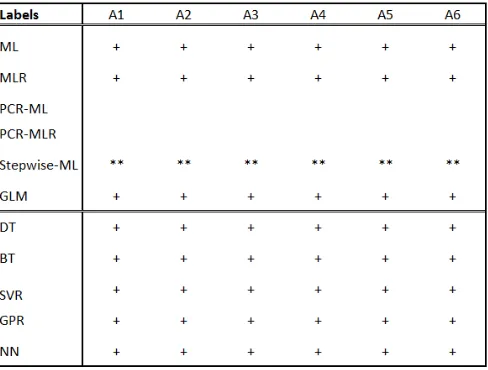
In our study of NIM forecasting models, we examine 10 Linear Regression models with the Standard Feature Selections labelled by FS1-FS10 in Table 1; in addition, we looked into 6 other feature selections, which are labelled by A1−A6 in Table 5 and which correspond with the quadratic terms of FS5-FS10
respectively as described in details in Appendix A.2. Altogether, we investigated 16 ML models for studying forecast accuracy by benchmarking against the random-walk baseline.
2.2.2 Multiple Linear Robust Regression Model or MLR
As highlighted in literature (e.g. Fox and Weisburg, 2013), the LS estimator can behave badly when error distributions are not normal, particularly when the probability distribution of the errors is heavy-tailed. Outliers can be informally defined as data points which are inconsistent with a (presumed) general trend. Outlying feature- or dependent variables can significantly influence the LS estimator, particularly for finite samples of moderate size, since residuals are equally weighted and squared. In the presence of outliers, one strategy is to remove them entirely from the sample, but this requires some criterion of when a data point can be considered to be an outlier. Another strategy is to use Robust Regression with the aim to down-weight the influences of possible outliers. Huber (1964) introduced a general so-calledM-estimator (owing to its similarity with Maximum Likelihood Estimation or MLE), which includes the LS estimator as a special case. In our study, we apply Robust Regression to the Linear Regression model, to which we refer as the MLR Model.
If we define the residual term ei for data point ias ei := yi−ξibb, the generalM-estimator proposed
by Huber minimizes a loss functionL := Pn
i=1ρ(ei) across allndata points for some given functionρ.In
particular, the LS estimator becomes a special case of theM-estimator by settingρ(ei)= e2
i. The function
ρ(u) should have the following properties:
• ρ is twice continuously differentiable, symmetric: ρ(−u)= ρ(u), and strictly increasing whenu > 0
withρ(0)=0.
• In particular, ρ(u) has a unique global minimum equal to 0 whenu = 0, and its derivativeφ(u) :=
∂ρ
∂u(u)>0 whenu>0 whileφ(u)<0 whenu<0.
Clearly, LS estimator satisfies the above properties, we can minimize L = P
i(yi−ξib)2 by setting its partial derivatives with respect to each component ofbequal to 0, which leads to the system ofkequations (wherekcoincides with the dimension of parameter vectorb, in particular,k=d+2 as indicated above):
m
X
i=1
φ(ei)ξi,j=0 for j=1, . . . ,k. (7)
Introducing weightswibywi:= φ (ei)
ei ifei,0 while settingwi=ρ
00
(0) ifei=0, we can rewrite this system as
m
X
i=1
(wiei)ξi,j= n
X
i=1
wi(yi−ξib)ξi,j=0 forj=1, . . . ,k. (8)
Note that, on account of the sign ofφ(u) for positive and negativeu,φ(u)/u>0, the weights are positive. After some manipulations and lettingWbe the diagonal matrix with the weightswion the diagonal, equation (8) is equivalent to
b=[ΞTWΞ]−1ΞTWy, (9)
whereΞis then×k-matrix (ξi,j) and yis the response vectory = (y1, . . . ,yn).Equation (9) resembles the
solution of a Weighted LS estimator problem minimizingL=P
(wiei)2, but note that the matrixWdepends on the residualsei, and therefore onb, so this is actually a system of non-linear equations for the components ofb.This system can be solved iteratively as follows: let us definew(u) :=φ(u)/uforu,0, andw(0)=φ0(0),
so thatwi=w(ei).Then:
1. Initializeb=b0by takingb0the LS estimator (6).
2. Usingb0, compute the regression errorse0
i =yi−ξib
0and from that the weight matrixW0:=diag(w(e0 i)) andb1:=[ΞTW0Ξ]−1ΞTW0y.
3. Iteratively, forν≥2, givenbν−1,
• Fori=1, . . . ,m, computewν−1
i :=w(eν
−1
i ) whereeν −1
i :=yi−ξibν
−1, and putWν−1=diag(wν−1
Figure 1: Outliers for 6 Bank-specific NIMs in Data Sample
• Definebνby
bν=[ΞTWν−1Ξ]−1ΞTWν−1y. (10)
Step 3 is repeated until meeting some tolerance criterion, at which point we setbb≈bν.
The above algorithm starts with LS estimator, then iteratively weighs the error terms until the estimator converges. Consequently, it is known as theIteratively Reweighed Least Square or IRLSmethod. For our study we used Tukey’sbi-square weight function, defined by
w(e)=
(
[1−(e
K)
2]2 for|e|6K; 0 for|e|>K.
with a tuning constantK = 4.685, which is shown to be able to retain 95% efficiency of LS Estimator by Tukey (1977).
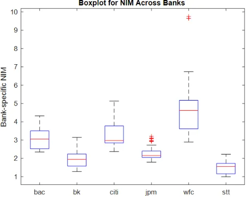
In Figure 1, we use boxplot to show the empirical distributions for the NIMs of the six G-SIBs investigated in our study; we note that each bank is distinguished by its stock ticker, which one can refer to Table 3 for the corresponding names associated with their stock tickers. Clearly, the NIMs for both ’jpm’ and ’wfc’ (indicating JP Morgan Chase and Wells Fargo banks respectively) have outliers indicated by ”+” highlighted in red colours. In this exercise, we adopt the definition ofoutlieraccording to Tukey (1977): outliers refer to data lying outside the so-called ”Tukey Fences”, i.e., the range defined as [Q1−k(Q3−Q1),Q3+k(Q3−Q1)] whereQ1andQ3denote the 25thand the 75thquantile respectively, andkis a constant. Tukey recommends to takek=1.5.Clearly, the NIM distributions for ”citi”, ”jpm” and ”wfc” are all positively skewed while only ”jpm” and ”wfc” have outliers.
We implement 10 MLR models corresponding with feature variables FS1-FS10, as shown in Table 1. Additional 6 models based on derived feature variables from standard feature variables can be found in Appendix A.2. As shown in our empirical section 3, the use of Robust Regression is conducive to improve the resistance against the influence on forecast accuracies from data outliers.
2.3
Principal Component Regression
variables: the principal components from Bolotnyy, Edge and Guerrieri’s were extracted from interest-rate only variables, whereas those of Grover and McCracken’s study were extracted from a diverse range of Macroeconomic variables, which might explains the divergence in their findings. One objective of our study is to investigate whether or not PCR-based Bank-specific NIM models can forecast significantly better than the Random Walk model. We also investigate the predictive performances with regard to varying the numbermof retained of Principal Components or PCs in the PCR model. Brummelhuis and Luo (2019a) uses Principal Component Analysis (or simply PCA) as a tool to investigate the potential impacts of Feature Correlations on Classification for a wide range of Classifiers.
More formally, we apply PC analysis to the ML or MLR model of sections 2.2.1 and 2.2 by replacing the feature variablesXd
twith a certain numbermof retained PCs extracted fromXdt: see Appendix A.3 for details. The resulting models will be denoted by PCR-ML and PCR-MLR respectively. In our study, we applied these two classes of models to NIM forecasting and investigated their forecasting performances when varying the numbermof PCs between 3 to 11 (the maximum number of raw feature variables). It is well-known that for yield-curve data, PC analysis withm=3 gives reasonably good results with a good interpretation for the extracted Principals. For illustration, we present in Appendix A.3 the PC components extracted from the US and the UK government yield curves based on data from 2000Q1 and 2016Q4. As indicated by our empirical results in section 3, increasingmdoes not necessarily lead to improved forecasting performances for PCR-based NIM Models because a largermonly means that a higher percentage of variance is explained by the retained PCs, but does not necessarily lead to higher forecasting accuracy. A similar phenomenon has been observed in Brummelhuis and Luo (2019a).
2.4
Generalized Linear Model or GLM
A linear model with response variableyand vector of explanatory variablesξcan be formulated as
E(y|ξ)=ξb,
wherebis the vector of parameters which have to be estimated. It has the property thatyis Gaussian ifξis multi-variate Gaussian. Such a model would not be appropriate if, for example, the values of the response variable would have to be restricted to some subdomain of the real numbers. An example in Finance is the modelling of default probabilities, whose values have to lie in the interval [0,1].In such situations a Generalized Linear Model or GLM might be more suitable. For such models one assumes thaty, conditional onξ, has a distribution in some given class of distributions, and that some suitable non-linear functiongof the conditional mean ofyis a linear function ofξ:
g E(y|ξ)=ξb.
The function g, which is called the link-function of the GLM, is chosen appropriately depending on the chosen class of distributions. As for us relevant example is the GLM-Gamma model, for which y|ξ is
assumed to follow a Gamma-distribution,
y|ξ∼ 1
θkΓ(k)y
k−1e−y/θ,
with parameterskandθand mean iskθ.The choice of link functiong(µ)=1/µ, leads to the conditional pdf:
kk(bTξ)k
Γ(k) e −k(ξb)y.
Given a sample (yi, ξi) and suitable distributional assumptions onξ, one can then write down the likelihood function and determine the parameters by Maximum Likelihood, in particular the vectorb(but also thek.) Forecasting is then simply done by inverting the regression equation above:
E(y|ξ)=g−1(ξb).
Figure 2: Summary for Performances by RMSE for Linear Models
2.5
An example: Using Linear models for NIM forecasting
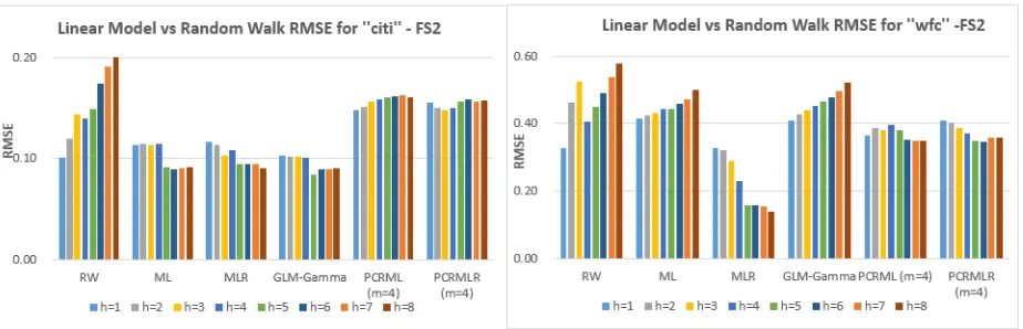
We end our discussion of linear models with an illustrative example. Figure 2 presents the root mean square (forecasting) errors (RMSE) for two banks, Citi Group Bank (”citi”) and Wells Fargo Bank (”wfc”), under the five linear models, ML, MLR, PCR-ML, PCR-MLR and GLM-Gamma, alongside with the benchmark RW model. All models were trained with the feature variable selection FS2 of Appendix A, and we used 4 principal components (orm= 4) for the PCR models. We see that the PCR-ML and PCR-MLR did not significantly outperform the RW model; while the MLR did in both cases of ”citi” and ”wfc”, the ML only outperformed in the case of ”citi”. As shown in Figure 1, the NIM data for ”citi” have no outliers, whereas those for ”wfc” do, which suggests that the use of Robust Regression can significantly enhance forecasting performance in the presence of outliers.
The choice of the RMSE as a metric to compare forecasting performances for different banks could be criticized on the grounds that it is scale-dependent. Figure 1, however, shows that the NIMs of ”citi” and ”wfc” are of comparable sizes. We have nevertheless also used scale-independent error measures for this study, which will be further discussed in section 2.11 below.
2.6
Stepwise Regression
Stepwise Regression is a technique for selecting the ”best” subset of feature variables out of a list of ”candidate” feature variables (and their transformations) based on a pre-specified criterion as a result of training a sequence of regression models. Stepwise Regression can lead to different choices of Feature Selections depending on the choices of criteria; in this study, we explore the choices of criteria such as Bayesian Information Criterion (BIC), Akaike information criterion (or AIC) and Sum of Squared Errors (or SSE), for which definitions are available from Hastie, Tibshirani and Friedman.
In this study, we focus on using Stepwise Regression in combination with ML model from the list of Feature Selections available in Appendix??. Stepwise Regression can be used in combination with GLM and other models but it is not in our scope. Therefore, although we present the performance for Stepwise Regression together with the rest of other models in Section 3, the fair performance comparison that one should conduct is between Stepwise and ML models because both are based on the same modelling set-up, i.e., ML.
2.7
Tree-based Regression Models
than by usingK-fold Cross Validation as we did in Brummelhuis and Luo (2019a), our data only being quarterly.
2.7.1 Regression Tree Models
Compared with the Linear Models discussed before, the Regression Tree model constructs a piecewise constant predictor function in which at each node of a decision tree, a constant sample mean of the target variable is fitted. Classification and Regression Tree or CART algorithms were introduced by Breiman, Friedman and Stone (1984). Classification Trees were for example used in Brummelhuis et al (2019a) for the construction of proxy CDS Rates.
In this paper, we adopt the Binary Regression Tree, in which the objective is to minimize the Sum of Squared (Forecasting) Errors or SSE, where the Forecasting Error is defined as the difference between the observed NIM and forecasted NIM within different partitioned regions of Feature Space. The forecasted NIM for each region will simply be the mean of the target variableyifor the data whose feature variables lie in that region. The different regions are rectangular boxes in feature space with faces parallel to the axes, and are obtained recursively by performing a succession ofsplits: given a feature variable, we can split our set of training data into two subsets, one where the chosen feature variable is smaller than some numberc, and one where it is bigger. Only finitely many such splits are possible, since the set of training data is finite. Calling the two subsetsLsandRs, where the subscriptsindicates the split, the SSE associated to the splits is defined by
s=
X
i∈Ls
(yi−µLS)
2+X
i∈Rs
(yi−µRs)
2, (11)
whereµLs = (#Ls)
−1P
i∈Lsyi and similarly for µRs.We then construct our tree by using a ”greedy” search
algorithm, starting offwith the entire training set at the base node, with its associated mean and SSE, and recursively choosing splits which minimize the total SSE, creating two new nodes of the tree for each such split. The algorithm stops splitting if the resulting tree meets certain constraints, such as the SSE becoming smaller than some pre-assigned number or by imposing a constraint on the maximum number of splits. This is known asStandard CART. There are two other variants, Curvature Test CART andInteractive Test CART, which we briefly describe.
Standard CART treats all predictor splitting homogeneously in terms of their influences on the target variable. The Curvature Testand the Interactive Test, as proposed by Loh (2002), allow users to select a subset of feature variables based on (Pearson) Chi-square tests while respectively taking into account the heterogeneous Feature Influence on the target variable and the interactions between feature variables when they choose predictor splitting.
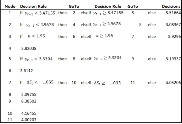
For this study, we tested a total of 10 Standard Regression Tree models, one for each Feature Selection (FS1-FS10) and implemented six additional models with feature selections FS5-FS10 to investigate heterogeneity of feature variable influence and its impact on NIM prediction, using theCurvature Testand theInteraction Testdescribed above. Table 2 presents an illustrative example for NIM forecasting for the Bank of America (bac) using Standard CART with Feature Selection FS1, where we refer Appendix A.1 for the notations used. It is well-known that the Regression Tree is a weak learner, in the sense that it tends to over-fit a given set of training data, and that its forecasting performance on other data sets then is not very good. This is sometimes called the generalization problem. With the hope to improve the robustness of a Regression Tree’s forecasts we use Ensemble learning, where we train an ensemble of Regression Trees instead of a single one.
2.7.2 Ensemble/Bagged Regression Trees or B-Tree
Ensemble Learning is a general Machine Learning philosophy in which, using techniques such as Boot-strapped Aggregation (or Bagging), Boosting or Random Forest, one combines the outcomes from several weak learners to arrive at a final learning outcome which is expected to be stable in the sense of reducing the variance. We focus on Bagged Regression Trees and refer the interested reader to Hastie, Tibshirani and Friedman for a detailed discussion of the other two techniques, which we haven’t employed for this study.
Table 2: A Simple Illustrative Example for Regression Tree results (’bac’ learned under FS1)
1. First, we draw random samples with replacement from the training dataDTto create a new training sets byDT∗
b , to which is often referred as a bag, whereb=1, . . . ,Band eachD T∗
b can have some rows repeated or some rows missing fromDT.
2. Second, for eachb=1, . . . ,Bwe train a Regression Tree based onDT∗
b , thereby obtaining a predicted value denoted asyb∗
bassociated with bagb.
3. Finally, we define the forecasted value for the Bagged Regression Tree as the average of the forecasted values fromBbags.
by=
1
B
B
X
b=1
b
y∗
b (12)
In our study, we use the Bagged Trees (or called B-Tree) by growing Regression Trees as described in Section 2.7.1. The motivation to use Bagged Regression Trees is to minimize the variance of prediction errors in least square sense across different Regression Trees and mitigate the so-called generalization problem associated with single Decision Tree.
2.8
Support Vector Regression or SVR
Support Vector Machines (SVM), introduced by Cortes and Vapnik (1995), can be used for both classification and regression. For a two-class classification problem with linearly separable data, the basic idea is to construct a separating hyperplane which is at maximum distance of both classes, equivalently, which creates a maximal margin, to ensure stability with respect to generalization. The same idea underlies SV Regression: see for example Sch ¨olkopf and Smola (1998). In linearε-SV regression one looks for a linear function f(x) =βTx+β
0 such that|yi− f(xi)| ≤ ε, for all pairs (xi,yi) in the training set and such that the distances of the (xi,yi) to the hyperplane defined by f are as large as possible. Since this distance can be shown to be equal to|yi−(βTxi+β0)|/p1+||β||2 with||β||2 = βTβthe Euclidean norm, and the numerator is bounded byε, one therefore wants to minimize||β||2.This leads to a constrained minimization problem.
In the literature one often encounters the phrase that one is looking for a linear function f which is ”as flat as possible”, a terminology which may be confusing (since any hyperplane is after all flat) unless this is interpreted as ”as horizontal as possible”. Another motivation for wanting to have||β||as small as possible
As it stands, this problem may not be feasible, for there may not exist a (β, β0) such that the constraints |yi− f(xi)| ≤εare satisfied for all elements of our training set. We therefore allow, as for the ”soft-margin”
version of the SVM classifier, that these constraints can be violated but at a cost proportional to the size of the violation. This leads to the following constrained minimization problem (Vapnik, 1995):
minβ12βTβ+CPiN=1(ξi+ξ∗i) subject to
∀i:yi−βTx
i+β0)6+ξi,
∀i: (βTxT
i +β0)−yi6+ξ
∗ i,
∀i:ξ∗ i >0,
∀i:ξi>0.
(13)
In Non-linear SV Regression one first transforms the feature variables via an invertible non-linear map
ϕ(x) of feature space to some higher-dimensional space, and then performs a linear SV Regression on the transformed data points (ϕ(xi),yi).It turns out that the algorithm for linear regression can be formulated completely in terms of the scalar productsxT
ixj, and we therefore only needk(xi,xj), wherek(x,z) :=ϕ(x)
Tϕ(z), the so-called kernel function. The functionk(x,z) is positive definite, and any such a positive definite function comes from a suitable transformationϕ, by a mathematical result known as Mercer’s theorem. It therefore suffices to specifykand keep the underlying transformationϕimplicit. Examples of positive definitek’s are Gaussian and homogeneous polynomials inxTz.For both Linear and Non-linear SVR we only need to solve a quadratic optimization problem, for which numerical solvers are readily available from a variety of statistical or numerical computational packages.
In our study we set the parameterCin (13) equal toC:= IQR1.3490(y), whereIQR(y) stands for the Inter-quartile range11or IQR of theyi, and 1.3490 is the IQR of the standard normal distribution. The loss-tolerance level was set equal to one-tenth of the standardized IQR:= IQR13.490(y).We used the Sequential Minimal Optimization algorithm or SMO, of Platt (1998), which is provided in standard software, as our solver. We experimented with two different Kernel functions, the Gaussian,k(x,y)=e−||x−y||2/σ2
, and the Linear kernel,k(x,y)=hx,yi
and used the kernel bandwidthσ chosen heuristically based on the median distance between a training point and its nearest neighbour, as described in Kim and Scott (2012).
2.9
Gaussian Process Regression or GPR
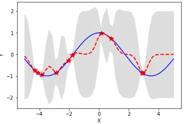
Given a training setDT ={(x
i,yi) :i=1,· · ·,n}of data, we want to predict the valuesy∗i for a set of feature variables{x∗
i}different from thexi’s which appear in the training set. The basic idea of Gaussian Process Regression or GPR, which first appeared in Danie G. Krige’s master thesis in the area of Geostatistics (which is why GPR is also called Kriging12, and was subsequently formalized by the French mathematician George Matheron (1963) is that, rather than doing this by fitting some parametric function f to the data setDTand subsequently using that function for prediction, we put an appropriate probability measure on the set of all functions, and predict the new values as a conditional expectation:
y∗i =E
f(x∗i)|f(xi)=yi,i=1, . . . ,n.
The probability measure is specified by requiring that for any set of pointsx1, . . . ,xpof feature space, the vector of function values (f(x1),· · ·,f(xn)) should be multivariate normally distributed (remember that here it is f which is random). A normal distribution is uniquely characterized by its mean, which in this context is usually taken to be 0, and its variance-covariance matrix, which is made up of the two-point covariances
k(xi,xj) = E
f(xi)f(xj)(given the zero-mean assumption), so we only need to specify the latter. In fact,
any kernel functionk(x,x0
) which is positive definite13can be chosen as correlation function. Given such a positive definite kernel function, we define a Gaussian process (or Gaussian field) onRnby specifying that
f(x1), . . . ,f(xn)∼N(0,K(X,X) ), (14)
11defined as the difference between the upper and lower quartiles
12Krige, D., ”Gaussian Process Regression”, Wikipediahttps://bit.ly/2zHkRkc 13In the sense thatPn