Sphere-Tree Construction using Dynamic Medial Axis Approximation
Gareth Bradshaw and Carol O’Sullivan Image Synthesis Group, Dept. of Computer Science,
Trinity College, Dublin, IRELAND
{Gareth.Bradshaw, Carol.OSullivan}@cs.tcd.ie
Abstract
Collision handling is very computationally expensive, especially in large scale interactive animations. Hierarchical object representa-tions play an important role in performing efficient collision han-dling. Many different geometric primitives have been used to con-struct these representations, which allow areas of interaction to be localised quickly. For time-critical algorithms, such as interrupt-ible collision detection, there are distinct advantages to using hier-archies of spheres, known as sphere-trees. This paper presents a novel algorithm for the construction of sphere-trees. The algorithm presented approximates objects, both convex and non-convex, with a higher degree of fit than existing algorithms. In the lower levels of the representations, there is almost an order of magnitude decrease in the number of spheres required to represent the objects to a given accuracy.
CR Categories: I.3.5 [Computer Graphics]: Computational Ge-ometry and Object Modeling—Object hierarchies; I.3.7 [Computer Graphics]: Three-Dimensional Graphics and Realism—Animation G.1.2 [Mathematics of Computing]: Numerical Analysis— Approximation
Keywords: sphere-tree construction, object approximation, me-dial axis, level-of-detail collision detection
1
Introduction
Collision handling is a major bottleneck in any interactive sim-ulation. Ensuring objects interact in the correct manner is very computationally intensive and much research has addressed the is-sues involved with trying to reduce the computational requirements. Researchers often utilise hybrid collision detection algorithms to tackle the problem in various phases. The initial phase of such an algorithm, known as the broad phase, aims to efficiently cull out pairs of objects which cannot possibly be interacting. A number of different techniques have been used to achieve this coarse grain de-tection. These include Sweep & Prune [Cohen et al. 1995; Ponamgi et al. 1997], global bounding volume tables [Palmer and Grimsdale 1995] and overlap tables [Wilson et al. 1998].
Having determined which objects are potentially interacting, the hybrid algorithm uses a finer grained algorithm to narrow in on the
regions of the objects which are in contact. This narrow phase pro-cessing typically traverses hierarchical representations of the ob-jects to hone in on the regions of interest. This reduces the amount of work that is required to perform the “exact” collision detection using such algorithms as Lin-Canny [Lin and Canny 1991; Lin 1993], V-Clip [Mirtich 1998] or Enhanced GJK [Gilbert et al. 1988; Rabbitz 1994; Cameron 1997].
Many different geometric primitives have been used for con-structing the “Bounding Volume Hierarchies” (BVH) used to per-form narrow phase processing. These include: Spheres [Quin-lan 1994; Palmer and Grimsdale 1995; Hubbard 1995a; Hubbard 1995b; Hubbard 1995c; Hubbard 1996; O’Sullivan and Dingliana 1999], Axis Aligned Bounding Boxes (AABB) [van Den Bergen 1997], Oriented Bounding Boxes (OBB) [Gottschalk et al. 1996; Krishnan et al. 1998a], Discrete Oriented Polytopes (k-DOP) [Klosowski et al. 1998], Quantised Orientation Slabs with Pri-mary Orientations (QuOSPO) [He 1999], Spherical Shells [Krish-nan et al. 1998b] and Sphere Swept Volumes (SSV) [Larsen et al. 1999].
There is often a trade-off between the complexity of the bound-ing volume primitive and the tightness of fit that can be achieved. Simpler primitives, such as spheres and AABBs, are quite inexpen-sive to test for intersections. However, as they provide relatively poor approximations, large numbers are often required to approxi-mate the objects effectively. More complex bounding volume prim-itives require more expensive intersection tests but, as they often provide tighter approximations, fewer primitives (and hence inter-section tests) are required. The following equation has been used in [Gottschalk et al. 1996], [van Den Bergen 1997] and [Klosowski et al. 1998] to evaluate various types of bounding volume hierar-chies :
T=Nu×Cu+Nv×Cv, (1)
where :
T is the total cost of collision detection between two objects,
Nu is the number of primitives updated dur-ing the traversal,
Cu is the cost of updating a primitive’s po-sition/orientation,
Nv is the number of overlap tests per-formed,
Cv is the cost of an overlap test between a pair of primitives.
Although spheres often do not provide particularly tight bound-ing volumes, there are a number of distinct advantages to their use. They are particularly advantageous when using the interrupt-ible collision detection algorithm. This algorithm, introduced by Hubbard, uses a time-critical traversal of the sphere-trees which is terminated when the allotted time-slice has expired so as to main-tain a consistent frame-rate [Hubbard 1995a; Hubbard 1995b; Hub-bard 1995c; HubHub-bard 1996]. As the collisions may never be re-solved down to the surface of the objects, the spheres can be used
Copyright © 2002 by the Association for Computing Machinery, Inc.
to approximate the collisions and formulate the response, as done in [O’Sullivan and Dingliana 1999; Dingliana and O’Sullivan 2000]. Attractive properties include :
• Rotational Invariance : A sphere is invariant to the rotation of the objects and therefore its update cost is very small. No matter what type of motion the bodies are going through the spheres can be updated by simply translating their centers.
• Efficient : The cost of performing an overlap test between two spheres is extremely low, requiring only a few floating point multiplications and additions.
• Suitability for Response : While providing graceful degrada-tion of the object approximadegrada-tion, each level of spheres in the hierarchy provides an approximation of the contact informa-tion necessary for collision response.
While many techniques have been used for the construction of sphere-trees, using the object’s medial axis (“skeleton”) has been shown to produce tight fitting sphere-trees. This paper presents a novel sphere-tree construction algorithm which extends the medial axis based algorithm to allow the medial axis to be constructed as required (full details can be found in [Bradshaw 2001]). Thus the medial axis always provides enough information for the construc-tion of the approximaconstruc-tion. The rest of this paper is organised as follows : Section 2 discusses the requirements of a good bounding volume hierarchy and gives a brief overview of some of the existing algorithms for the construction of sphere-trees. Section 3 overviews the process of sphere-tree construction within our frame-work and discusses how object sub-division is managed. Section 4 details the use of Voronoi diagrams for the approximation of the medial axis. Section 5 presents the adaptive medial axis approximation al-gorithm which extends the existing alal-gorithm to allow the approx-imation to be updated as required. Section 6 presents a number of new algorithms for the generation of sphere sets from the medial axis approximation. Section 7 evaluates the new algorithms for the approximation of objects, the construction of sphere-trees and their use within interactive simulations. Finally, Section 8 presents con-clusions and mentions some possible routes for future work.
2
Existing Algorithms
A number of algorithms have been used for the construction of sphere-trees. Any algorithm which constructs bounding volume hi-erarchies for collision detection must meet four basic requirements [Hubbard 1995b] :
• the hierarchy conservatively approximates the volume of the object, each level representing a tighter fit than its parent;
• for any node in the hierarchy, its children should cover the parts of the object covered by the parent node;
• the hierarchy should be created in a predictable automatic manner, not requiring user interaction;
• the bounding volumes within the hierarchy should fit the orig-inal model as tightly as possible, representing it to a high de-gree of accuracy.
For interactive simulations, the emphasis is on achieving high and consistent frame-rates. Therefore a major concern is how well the hierarchy facilitates this goal. As the collision detection algo-rithm may not fully resolve the collisions, approximate collision information must be available from each level of the BVH.
The simplest algorithm for construction of sphere-trees uses the octree data-structure. The sphetree is constructed by using re-cursive sub-division of the object’s bounding cube. The regions which cover part of the object are then further sub-divided, continu-ing down to the required depth. The sphere-tree is then constructed by placing a sphere around each of the nodes of the octree. This method has been adopted in [Palmer and Grimsdale 1995; Hubbard 1995a; Hubbard 1995b; Hubbard 1996; O’Sullivan and Dingliana 1999]. The simplicity of the algorithm allows it to be quickly and easily implemented and for the sphere-trees to be updated when objects deform. However, the sphere-trees produced often fit the object quite poorly.
Quinlan also uses sphere-trees for collision detection. The sphere-trees are constructed by first covering the surface with a set of uniformly sized spheres which represent the leaf nodes of the hierarchy. This set of spheres is divided into two (roughly equal) sub-sets. Trees are constructed for each of the two sets and these trees are used as children of the root [Quinlan 1994]. Q-Splat uses a similar strategy for constructing sphere-trees for visibility culling and level-of-detail rendering [Rusinkiewicz and Levoy 2000].
Along with the octree method, Hubbard also explored two other methods for the construction of sphere-trees. He initially used
sim-ulated annealing for sphere-tree construction. Later he used the
object’s medial axis to guide where to put spheres. This method provides tight fitting sets of spheres from which the sphere-tree is constructed.
3
High-Level Construction Algorithm
This section gives an overview of the new sphere-tree construction algorithm. The algorithm consists of a number of layers. The top layer decomposes the construction into a number of sub-problems. It controls how the object is sub-divided into regions, each of which needs to be approximated with a set of spheres. These spheres will become the children of the sphere which was used to define the approximated region.
The root node of the sphere-tree is the smallest sphere that will enclose the object, which can be found with a minimum enclos-ing ball algorithm [Weltz 1991; White (www)]. The first level of spheres, the children of the root sphere, are constructed by calling a sphere generation algorithm which generates the required number of spheres to cover the object. These spheres are then used to seg-ment the object into a number of regions. Each region defines the areas of the object that must be covered by a set of children spheres. These spheres form the next level of the hierarchy - as children of the sphere that defined the region.
3.1 Object Segmentation
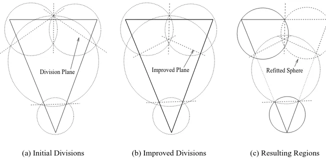
Division Plane
(a) Initial Divisions
Improved Plane
(b) Improved Divisions
Refitted Sphere
[image:3.597.137.463.48.207.2](c) Resulting Regions
Figure 1: Dividing the object into distinct regions using dividing planes.
Rather than working directly with the underlying model, the sur-face is represented by an arbitrarily large set of sample points. Thus to segment the object into regions we simply choose the sub-set of points that represent the surface within that area. For points cov-ered by many spheres it is necessary to assign the point to one of the sets of children. This is achieved by dividing the overlapping region between the spheres. For each pair of overlapping spheres a dividing plane is constructed. The points contained within the in-tersection of the two spheres are divided based on which side of the plane they lie on.
Figure 1 shows how a triangular object is divided into four re-gions. The dividing planes, shown in Figure 1(a), are constructed so that the plane passes through the points of intersection of the spheres (circles in 2D). In this example the region associated with the large central sphere is much bigger than the regions associated with the other spheres. Thus, the children of this sphere will poten-tially have a looser fit than the other child sets. It is very desirable that the regions divide the object as evenly as possible without af-fecting the fit of the current set of spheres. Thus, the dividing plane between a pair of spheres is moved to try to get each to cover a region of equal size, Figure 1(b). Once we have established the regions to be covered by each of the spheres, new spheres can be created. These new spheres are now only required to cover the parts of the surface which are not covered by any other spheres, allowing a tighter sphere to be fitted, Figure 1(c).
4
Medial Axis Approximation
Constructing the medial axis for a polyhedral model is a compli-cated and computationally expensive task. For the purposes of con-structing sphere-trees an approximate medial axis suffices. This section describes the algorithm for constructing a medial approxi-mation using a Voronoi diagram.
A Voronoi diagram is constructed from a set of forming points. Each cell within the Voronoi diagram represents the region of space which is closer to its forming point than any of the other forming points. When the set of points is distributed over the surface of the object, a sub-set of the faces that lie between the cells forms an approximation of the medial axis [Hubbard 1995b]. We use Hub-bard’s algorithm, based on work described in [Bowyer 1981] and [Inagaki et al. 1992], for constructing the Voronoi diagram.
The algorithm for the construction of the Voronoi diagram is an iterative one. Each of the forming points, which are points dis-tributed across the surface of the object, is added to the diagram in
turn. As the points are added, new cells are constructed and the ex-isting cells are updated so that each one still represents the region of space closest to its forming point. The algorithm is initialised with a Voronoi diagram containing 4 forming points which form a bounding tetrahedron for the object. The Voronoi vertices (which make up the cells) consist of one true vertex, constructed from the forming points, and 4 dummy vertices located at infinity.
When a new point is added to the Voronoi diagram, a new cell must be formed. This cell represents the region of space closer to the new forming point than to any of the existing forming points. To update the Voronoi diagram, the vertices which are closer to the new forming point need to be removed and new vertices created. Vertices which are approximately equidistant from both their form-ing points and the new point are considered marginally deletable. These are problematic as it is difficult to determine if they should be deleted or not. Hubbard finds the set of deletable vertices by considering the vertices in order of removability. The search starts with the most deletable vertex and maintains a priority queue of the possibly deletable vertices, which is initialised with the posi-tively valued neighbours of the starting vertex. Each vertex in the queue is considered in order of removability. If the deletion of a vertex will invalidate the Voronoi diagram, i.e. it cannot be added to the deletable set, it is held back for later consideration. When a deletable vertex is found, its positively valued neighbours are added to the priority queue, and the vertices that were being held back are returned to the queue for further consideration.
Having found the set of deletable vertices, a new vertex is created for each pair of neighbouring vertices Vd and Vu, where Vd is a deletable vertex and Vuis an undeletable vertex. These vertices will share three forming points, which together with the new point will create the new vertex. The circumcenter of the tetrahedron formed by these four points gives the vertex’s location. As with all Voronoi vertices, the new vertex Vnhas four neighbours, Vuand three other new vertices. These other neighbours are the new vertices with which it shares 3 forming points.
5
Adaptive Medial Axis Construction
The algorithm presented in the previous section approximates the medial axis of an object with a Voronoi diagram. There are, how-ever, a number of difficulties associated with this process. When generating the Voronoi diagram, it is difficult to choose the set of surface samples correctly. Problems in choosing the set of surface points can result in the medial axis being pushed through the sur-face to create either a hole in the approximation or a bridge that joins two separate areas of the object.
Hubbard introduces the notion of “gap crossing” cells as a way of identifying and fixing these problems [Hubbard 1995b]. How-ever, this scheme does not address the problems associated with constructing a sphere-tree from the medial axis approximation. It is impossible to determine a priori how to construct a medial axis, and hence the set of medial spheres, that will best suit the sphere-tree being constructed. We favour an adaptive medial axis construction algorithm, presented in this section. This algorithm handles both the gap crossing problems and allows the medial axis approxima-tion to be updated so that there is always a sufficient number of spheres available to construct the sphere-tree and to fit the object to a high degree of accuracy.
The adaptive medial axis approximation algorithm is iterative in nature. It starts with an empty Voronoi diagram and iteratively improves the approximation by adding new sample points to the surface of the object. The first task of the algorithm is to ensure that the set of medial spheres, which is the set of spheres placed around the Voronoi vertices, covers the object’s surface. The second phase of the adaptive algorithm is to adaptively improve the medial spheres.
5.1 Completing Coverage
In order to ensure that the set of medial spheres is complete, it must cover the entire surface. This is achieved by representing the ob-ject as a densely packed set of points distributed across its surface. The surface is considered to be covered when all these points are covered by spheres. This representation makes it simple to ensure that the model is completely covered. For those points which are not covered we need to create spheres which will cover them. As the set of spheres placed around a Voronoi cell’s vertices will cover every part of the cell, the extra spheres can be chosen from those belonging to the cell that contains the uncovered point.
There are several criteria that could be used to choose the sphere to cover each point. The smallest sphere, or the sphere with the lowest error, would help to produce a tight fitting approximation, whereas choosing the largest sphere would also cover a number of other uncovered points. This would mean that fewer of the spheres in the approximation would be “coverage spheres”. As the adaptive algorithm is able to replace poor fitting spheres, these spheres will subsequently be replaced if they affect the quality of the approxi-mation.
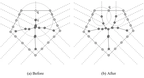
5.2 Iterative Improvement
The second phase of the adaptive medial axis approximation rithm is the improvement step. During each iteration of the algo-rithm, having marked the medial (and coverage) spheres, the sphere with the worst fit is replaced1. This is achieved by adding a new sample point to the Voronoi diagram. This point, q, is the point on the surface which is closest to the center of the sphere, c. As q will be closer to the vertex than its forming points, this results in the vertex being replaced with new ones, as illustrated in Figure 2.
1Each Voronoi vertex caches its sphere and the associated error to allow the worst fitting sphere to be chosen quickly.
6
Sphere Generation
The top level sphere-tree construction algorithm, presented in Sec-tion 3, expresses sphere-tree construcSec-tion as a number of sub-problems, each requiring that a region of the object be approxi-mated with a set of spheres. This section details the process of constructing sphere sets from the medial axis approximation.
The sphere generation algorithm maintains a Voronoi diagram which approximates the medial axis of the object. Prior to the con-struction of a set of spheres, the medial axis is updated so that it is of sufficient quality to allow a tight approximation. For this we re-quire that the set of spheres covering the region to be approximated contains some multiple of the target number of spheres and that the worst sphere in the set has an error which is a fraction (typically 12 to41) of the parent sphere’s error.
Having updated the medial axis approximation, the set of spheres which approximates the required region is used to construct the spheres for the sphere-tree. This set of spheres is reduced so that it contains the required number, i.e. equal to the branching factor of the tree. We have explored a number of algorithms for performing this reduction. Our favoured approach is to use two different algo-rithms, detailed next, and choose the set of spheres which best fits the object.
6.1 Merge
The “merge” sphere reduction algorithm, loosely based on Hub-bard’s algorithm, reduces the sub-set of medial spheres by succes-sively merging pairs of spheres. Each sphere is allowed to merge with a number of other spheres, its neighbours. Initially, each sphere is given a set of neighbours which correspond to the vertex’s neighbours within the Voronoi diagram.
Each of the medial spheres covers a sub-set of the surface points. When a pair of spheres is merged, a new sphere is constructed which covers the union of the two sets of surface points. When constructing this sphere we wish to keep it close to the medial axis. Thus we use two approaches to constructing the bounding sphere. We first resize both the spheres to enclose both sets of points. Next, we create the minimum volume bounding sphere for the points, us-ing White’s algorithm [White (www)]. The final sphere is chosen to be the one with the lowest error.
Having combined a pair of spheres, the set of merges is updated. The neighbours of each of the merged spheres will become neigh-bours of each other, resulting in new potential merges. Any spheres that end up with no neighbours are given an artificial set of neigh-bours. This set of neighbours consists of any spheres which overlap the neighbourless sphere or all the remaining spheres if there are no overlaps. The reason for limiting the pairs of spheres that may be combined is to reduce the computational cost of the reduction process. When the number of spheres becomes sufficiently low, it becomes feasible to consider every pair for merging. This is typi-cally done when we reach 2 or 3 times the target number of spheres. Each iteration of the merge algorithm reduces the number of spheres by one, using a greedy algorithm. At each iteration, the merge which results in the lowest error is used. This does not con-sider the effects of the merge on future operations. We give spe-cial consideration to merges which actually reduce the error in the approximation. We refer to these as “beneficial merges”. As an approximation is only as good as its worst error, we favour merges which improve the worst spheres in the approximation.
6.2 Expand
c q
(a) Before
q
[image:5.597.167.445.48.200.2](b) After
Figure 2: Addition of a new point to the Voronoi diagram to improve the approximation.
to choose a set of spheres that distribute the error evenly between them. By ensuring that all the spheres have the same error, the algo-rithm will have a better chance of achieving a tight fit. For a convex body, a sphere can be grown to hang over the surface by a given amount, e, using the following equation to calculate its radius (with
q and c as defined in Section 5.2) :
r=e− kq−ck (2)
Thus, the medial spheres are expanded to the desired stand-off distance, using Equation 2, and a sub-set of the spheres is se-lected. For non-convex bodies, the stand-off distance is an over-approximation of the error present in the sphere. A simple search al-gorithm, derived from binary search, is used to find the lowest value of e that results in a set that does not contain too many spheres.
The job of selecting the minimum number of expanded spheres that cover an object is a complicated one. Instead of looking for the globally optimum set we try to find a good minimal set of spheres, i.e. a set of spheres from which none of the spheres can be removed without exposing part of the surface. A greedy algorithm allows us to achieve this efficiently. In this algorithm the set of currently se-lected spheres is maintained and more spheres are sese-lected until the region is completely covered. To decide which sphere to add, each sphere is ranked according to its potential to keep the set of spheres small. Two heuristics for ranking the spheres have been explored. The first is to simply rank the spheres by the area of previously un-covered surface contained within it. The second heuristic ranks the spheres by the number of other spheres which it makes redundant. The second heuristic tends to select spheres near to those previously selected and seems to work slightly better in practice.
7
Evaluation
This section compares sphere-trees generated using the new algo-rithm with existing medial axis based sphere-trees. Other tech-niques, including the octree method, have also been evaluated but the results are not included here as the medial axis method produced far tighter fitting hierarchies, as expected. A full discussion of these and other results can be found in [Bradshaw 2001].
The algorithms have been compared using a number of simple geometric shapes including a cube, an ellipsoid, a cylinder, a torus, a cone, an S-shaped object and a block with square cross sections. A number of commonly used complex models have also been used,
including the Bunny2, the Cow and the Dragon3. The Bunny and S-shape are shown in Figure 3.
There are a number of factors which must be considered when approximating an object with spheres. As stated in Section 2, the spheres should approximate the object’s surface to a high degree of accuracy and should cover the entire object. The tightness of fit can be measured as the maximum distance from the surface of the spheres to the actual surface of the object. This represents an upper bound on the distance between two objects when they are falsely thought to be involved in a collision. The initial analysis is concerned with the geometric properties of sphere-trees and the later analysis considers the use of the resulting sphere-trees in an interruptible collision handling system.
7.1 Sphere-Tree Construction
Figure 4 compares the geometric fit achieved using the various sphere reduction algorithms. All tests were conducted with a tree branching factor of 8. All the algorithms used a set of 5000−10000 surface points to check coverage. The original algorithm was used with a medial axis approximation containing circa 2500 spheres. For the adaptive algorithm, the medial axis initially contained 500 spheres and was dynamically refined so that each region had 12 the error of the parent sphere and at least 100 spheres, i.e. the merge/expand algorithms started with 100 spheres from which the final 8 were to be produced.
The new merge algorithm shows significant improvements over the original algorithm. For complex models, such as the Bunny, the 3rdlevel spheres produced by the new merge algorithm exhibit about 12the error of those constructed with the original algorithm. The expand algorithm shows further improvements and using both sphere reduction algorithms in combination results in a further de-crease in error. In fact, the worst case for the combined algorithm’s level 2 spheres is roughly the same as that for the original algo-rithm’s level 3 spheres (see Figure 4(a)). Thus the combined al-gorithm produces the same tightness of fit using around 18ththe number of spheres.
7.2 Simulation
In order to further evaluate the sphere-tree generation algorithm, the behaviour of the sphere-trees during simulation was tested. During
2Data from http://graphics.stanford.edu/data/3Dscanrep/
(a) Bunny (b) S-shape
Figure 3: Some of the models used for testing the algorithms.
0 0.05 0.1 0.15 0.2 0.25 0.3 0.35 0.4 0.45
Level 1 Level 2 Level 3
Error
Hubbard Merge Expand Combined
(a) Bunny
0 0.05 0.1 0.15 0.2 0.25 0.3 0.35
Level 1 Level 2 Level 3
Error
Hubbard Merge Expand Combined
[image:6.597.125.494.288.440.2](b) S-Shape
Figure 4: Comparison of sphere-tree construction algorithms (worst error).
0.3 0.4 0.5 0.6 0.7 0.8 0.9 1 1.1 1.2
0 5000 10000 15000 20000 25000 30000
Fraction of Error
Interruption Interval Merge Expand Combined
(a) Worst Error
0.1 0.2 0.3 0.4 0.5 0.6 0.7 0.8 0.9 1 1.1
0 5000 10000 15000 20000 25000 30000
Fraction of Collisions
Interruption Interval Merge Expand Combined
(b) Resulting Contacts
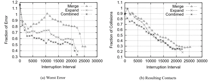
[image:6.597.100.505.492.652.2]these simulations, objects were positioned (and oriented) randomly about a sphere and given a random velocity towards a central point. Each sphere-tree approximation of the object was evaluated during the simulations. At each time-step the colliding pairs were created by testing their bounding spheres. The sphere-trees for these pairs were then traversed as they would be in the interruptible collision detection algorithm. To avoid bias towards or against a particular sphere-tree, the motions of the objects and their response to colli-sions were computed using a commercial dynamics system which uses an “exact” collision detection algorithm and a complex friction dynamics model.
The sphere-tree traversals were interrupted at regular intervals and the approximate collisions evaluated. The error associated with each colliding pair was computed as the sum of the spheres’ errors, i.e. the maximum distance between the sphere and the surface. This represents an upper-bound for the true separation between the ob-jects. The new algorithms were compared to a reference sphere-tree, i.e. that constructed with Hubbard’s original algorithm. For each interruption time, the average improvement was computed us-ing all the frames of the animation (typically 1000+).
Figure 5 presents results for simulations containing 20 objects. The horizontal axis of each of the graphs shows the interruption in-terval. This is expressed in terms of the number of primitive opera-tions performed, i.e. sphere updates and overlap tests. The amount of work done before interruption is computed using Equation 1. The values of Cuand Cvare 2 and 1 respectively. These values rep-resent the relative number of floating point operations performed when updating a sphere’s position (21 floating point operations) and testing two spheres for overlap (10 floating point operations). The first graph (a) in each set shows the fraction of error present in the approximations and the second (b) shows the relative number of colliding pairs produced by the different algorithms.
The new algorithms show a definite reduction in error. For com-plex models, such as the Bunny, the combined algorithm quickly falls to as little as 50% of the error resulting from existing algo-rithms (see Figure 5(a)). The amount of error continues to decrease to as low as 30%. In other simulations, using the simpler models, we have found this to be as low as 20%. The algorithms also show significant reductions in the numbers of pairs of colliding spheres, which result from the traversal. This provides a reduction in the amount of work which will need to be done by the later stages of the collision handling system, i.e. contact modelling and collision response. For the Bunny, the number of resulting collisions has decreased to as little as 20% (see Figure 5(b)).
8
Conclusions & Future Work
This paper has presented some novel work in the areas of medial axis approximation and sphere-tree construction. An adaptive me-dial axis approximation algorithm, which addresses many of the issues involved with using Voronoi diagrams for this purpose, was presented. The adaptive algorithm not only allows us to ensure that every part of the object is approximated but also allows the sphere-tree construction algorithm to refine the approximation as it moves down the sphere-tree. The approximate medial axis is then used to construct a set of spheres from which the sphere-tree is constructed. A generic sphere-tree construction algorithm was presented which expresses the task as a number of sub-problems. Each of these sub-problems involves approximating a region of the object with a desired number of spheres. This allows many different al-gorithms, each of which generate the required number of spheres from the medial axis approximation, to be slotted into the top-level algorithm. The sphere reduction algorithm presented combines two of the algorithms we have explored. The merge algorithm is generic in nature and is suitable for most scenarios. The expand algorithm takes a novel approach to sphere reduction. This algorithm reduces
the set of medial spheres by enlarging them and selecting a sub-set to cover the object. This produces spheres which distribute the er-ror evenly between them and often results in tighter fitting sets of spheres.
The sphere-reduction algorithms were used for the construction of sphere-trees to approximate a number of different models. The new algorithms consistently provide improvement over the existing algorithms. In the lower levels of the sphere-trees, the new com-bined algorithm required almost an order of magnitude less spheres. The sphere-trees were also evaluated for use in interruptible simula-tions. The sphere-trees constructed with the new algorithms showed a large decrease in error and resulted in far fewer pairs of colliding spheres.
There are a number of interesting areas of research that can build upon this work. To date, we have concentrated on fitting tight hier-archies of spheres to rigid bodies. This can, of course, be used for articulated objects too. However, further work would be required to make the algorithms suitable for use with deformable objects. Also, many objects contain large flat areas which are not well approxi-mated by spheres, e.g. buildings. For general purpose simulation it would be nice to be able to use other collision detection strategies for these areas while using sphere-trees where applicable. Sphere-trees have also recently been used for visibility culling and level-of-detail rendering [Rusinkiewicz and Levoy 2000; Rusinkiewicz and Levoy 2001]. It would be extremely interesting to combine this technique with level-of-detail collision detection so that the same sphetrees could be used for both. Finally, another interesting re-search area would be the construction of more generic bounding volume hierarchies containing many different types of primitive, each one being used where it is best suited.
References
BLUM, H., AND NAGEL, R. 1978. Shape description using weighted symmetric axis features. Pattern Recognition 10, 167– 180.
BOWYER, A. 1981. Computing Dirichlet tessellations. The
Com-puter Journal 24, 2, 162–166.
BRADSHAW, G. 2001. Bounding Volume Hierarchies for
Level-of-Detail Collision Handling. PhD thesis, Trinity College Dublin,
IRELAND.
CAMERON, S. 1997. Enhancing GJK: Computing minimum pen-etration distances between convex polyhedra. In Proceedings of
the Int. Conf. On Robotics and Automation, 3112–3117.
COHEN, J., LIN, M., MANOCHA, D.,ANDPONAMGI, M. 1995. I-COLLIDE: An interactive and exact collision detection system for large-scaled environments. In Proceedings of ACM Int.3D
Graphics Conference, 189–196.
DINGLIANA, J.,ANDO’SULLIVAN, C. 2000. Graceful degrada-tion of collision handling in physically based animadegrada-tion.
Com-puter Graphics Forum, (Proceedings, Eurographics 2000) 19, 3,
239–247.
GILBERT, E., JOHNSON, D., ANDKEERTHI, S. 1988. A fast procedure for computing the distance between complex objects in three-dimensional space. IEEE Transactions on Robotics and
Automation 4, 2, 193–203.
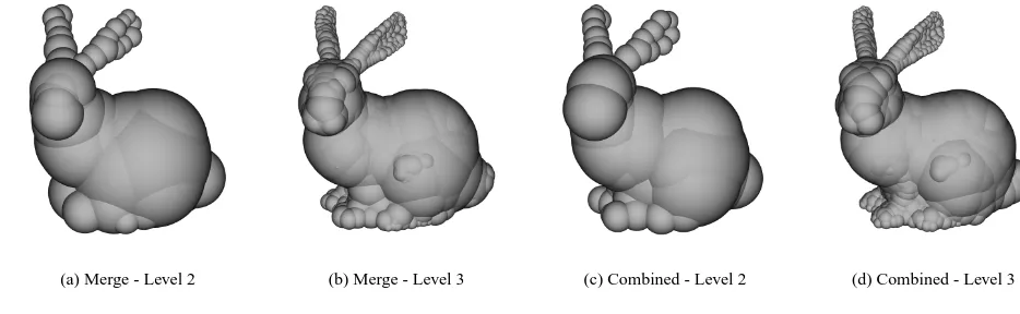
(a) Merge - Level 2 (b) Merge - Level 3 (c) Combined - Level 2 (d) Combined - Level 3
Figure 6: Sphere-trees constructed for the Bunny.
HE, T. 1999. Fast collision detection using QuOSPO trees. In
Proceedings of the 1999 Symposium on Interactive 3D graphics,
55–62.
HUBBARD, P. 1995. Collision detection for interactive graphics applications. IEEE Transactions on Visualization and Computer
Graphics 1, 3, 218–230.
HUBBARD, P. 1995. Collision Detection for Interactive Graphics
Applications. PhD thesis, Dept. of Computer Science, Brown
University.
HUBBARD, P. 1995. Real-time collision detection and time-critical computing. In Workshop On Simulation and Interation in Virtual
Environments.
HUBBARD, P. 1996. Approximating polyhedra with spheres for time-critical collision detection. ACM Transactions on Graphics
15, 3, 179–210.
INAGAKI, H., SUGIHARA, K., ANDN.SUGIE. 1992. Numeri-cally robust incremental algorithm for constructing 3D Voronoi diagrams. In Proceedings of the 4thCanadian Conference on Computational Geometry, 334–339.
KLOSOWSKI, J., HELD, M., MITCHELL, J., SOWIZRAL, H.,AND
ZIKAN, K. 1998. Efficient collision detection using bounding volume hierarchies of k-DOPs. IEEE transactions on
Visualiza-tion and Computer Graphics 4, 1, 21–36.
KRISHNAN, S., GOPI, M., LIN, M., MANOCHA, D., ANDPAT
-TEKAR, A. 1998. Rapid and accurate contact determination between spline models using ShellTrees. In Proceedings of
Eu-rographics ’98, vol. 17(3), 315–326.
KRISHNAN, S., PATTEKAR, A., LIN, M., ANDMANOCHA, D. 1998. Spherical shells: A higher order bounding volume for fast proximity queries. In Proceedings of the 1998 Workshop on the
Algorithmic Foundations of Robotics, 122–136.
LARSEN, E., GOTTSCHALK, S., LIN, M.,ANDMANOCHA, D. 1999. Fast proximity queries with swept sphere volumes. Tech. Rep. TR99-018, Dept. of Computer Science, University of North Carolina.
LIN, M.,ANDCANNY, J. 1991. Efficient algorithms for incremen-tal distance computation. In Proc. IEEE Conference on Robotics
and Automation, 1008–1014.
LIN, M. 1993. Efficient Collision Detection for Animation and
Robotics. PhD thesis, University of California, Berkeley.
MIRTICH, B. 1998. V-Clip: Fast and robust polyhedral collision detection. ACM Transactions on Graphics 17, 3, 177–208.
O’SULLIVAN, C.,ANDDINGLIANA, J. 1999. Realtime collision detection and response using sphere-trees. In Proceedings of the
Spring Conference on Computer Graphics, 83–92.
PALMER, I.,ANDGRIMSDALE, R. 1995. Collision detection for animation using sphere-trees. Computer Graphics Forum 14, 2, 105–116.
PONAMGI, M., MANOCHA, D., ANDLIN, M. 1997. Incremen-tal algorithms for collision detection between polygonal models.
IEEE Transactions on Visualization and Computer Graphics 2,
1, 51–64.
QUINLAN, S. 1994. Efficient distance computation between non-convex objects. In Proceedings International Conference on
Robotics and Automation, 3324–3329.
RABBITZ, R. 1994. Fast collision detection of moving convex polyhedra. In Graphics Gems IV, P. Heckbert, Ed. Academic Press, Cambridge, MA, 83–109.
RUSINKIEWICZ, S.,ANDLEVOY, M. 2000. QSplat: A multireso-lution point rendering system for large meshes. In Proceedings
of ACM SIGGRAPH 2000, ACM Press / ACM SIGGRAPH /
Addison Wesley Longman, K. Akeley, Ed., 343–352.
RUSINKIEWICZ, S.,ANDLEVOY, M. 2001. Streaming QSplat: A viewer for networked visualization of large, dense models. 2001
Symposium on Interactive 3D Graphics.
VANDENBERGEN, G. 1997. Efficient collision detection of com-plex deformable models using AABB trees. Journal of Graphics
Tools 2, 4, 1–13.
WELTZ, E. 1991. Smallest enclosing disks (balls and ellipsoids). In New Results and New Trends in Computer Science, H. Maurer, Ed. 359–370.
WHITE, D. (www). Smallest Enclosing Ball of Points/Balls.
http://vision.ucsd.edu/ dwhite/ball.html.