On the spatio temporal analysis of hydrological droughts from global hydrological models

doi:10.5194/hess-15-2963-2011

© Author(s) 2011. CC Attribution 3.0 License.

Earth System

Sciences

On the spatio-temporal analysis of hydrological droughts

from global hydrological models

G. A. Corzo Perez1, M. H. J. van Huijgevoort1, F. Voß2, and H. A. J. van Lanen1

1_{Hydrology and Quantitative Water Management Group, Centre for Water and Climate, Wageningen University,}

Droevendaalsesteeg 4, 6708 PB Wageningen, The Netherlands

2_{Center for Environmental Systems Research, University of Kassel, Kassel, Germany}

Received: 23 November 2010 – Published in Hydrol. Earth Syst. Sci. Discuss.: 19 January 2011 Revised: 24 August 2011 – Accepted: 24 August 2011 – Published: 19 September 2011

Abstract. The recent concerns for world-wide extreme events related to climate change have motivated the de-velopment of large scale models that simulate the global water cycle. In this context, analysis of hydrological ex-tremes is important and requires the adaptation of identi-fication methods used for river basin models. This paper presents two methodologies that extend the tools to analyze spatio-temporal drought development and characteristics us-ing large scale gridded time series of hydrometeorological data. The methodologies are classified as non-contiguous and contiguous drought area analyses (i.e. NCDA and CDA). The NCDA presents time series of percentages of areas in drought at the global scale and for pre-defined regions of known hydroclimatology. The CDA is introduced as a com-plementary method that generates information on the spa-tial coherence of drought events at the global scale. Spa-tial drought events are found through CDA by clustering patterns (contiguous areas). In this study the global hydro-logical model WaterGAP was used to illustrate the method-ology development. Global gridded time series of subsur-face runoff (resolution 0.5◦) simulated with the WaterGAP model from land points were used. The NCDA and CDA were developed to identify drought events in runoff. The percentages of area in drought calculated with both meth-ods show complementary information on the spatial and tem-poral events for the last decades of the 20th century. The NCDA provides relevant information on the average number of droughts, duration and severity (deficit volume) for pre-defined regions (globe, 2 selected hydroclimatic regions). Additionally, the CDA provides information on the number

Correspondence to: G. A. Corzo Perez ([email protected])

of spatially linked areas in drought, maximum spatial event and their geographic location on the globe. Some results cap-ture the overall spatio-temporal drought extremes over the last decades of the 20th century. Events like the El Ni˜no Southern Oscillation (ENSO) in South America and the pan-European drought in 1976 appeared clearly in both analy-ses. The methodologies introduced provide an important ba-sis for the global characterization of droughts, model inter-comparison of drought identified from global hydrological models and spatial event analyses.

1 Introduction

Drought is defined as a “sustained and regionally extensive occurrence of below average water availability” (Tallaksen and van Lanen, 2004). It is triggered by low or lack of rain-fall, often in combination with high evaporation rates. In regions with a cold climate, deviations from normal tem-peratures can also give rise to drought due to early snow accumulation or late snow melt (winter drought, van Loon et al., 2010). Different types of drought can be distinguished, i.e. meteorological drought, soil moisture drought and hy-drological drought (e.g. groundwater storage, river flow, lake storage) (e.g. Tallaksen and van Lanen, 2004; Wilhite, 2000; Heim Jr, 2002). Droughts have large socio-economic and environmental impacts affecting many sectors. Between 1991 and 2005, 950 million people were affected by droughts worldwide and an economic damage of 100 billion US dol-lars was reported (UN-ISDR, 2009). Data for Europe from 2000–2006 show that each year on average 15 % of the EU total area and 17 % of the EU total population have suf-fered from the impact of droughts. The estimated total costs

2964 G. A. Corzo Perez et al.: Spatio-temporal analysis of hydrological droughts of droughts for Europe over the past 30 years amount to

100 billion Euros (EC, 2007). Climate change projections in-dicate continental drying and a likely associated increase in dry spell length and frequency of drought over, for instance, many mid-latitude continental interiors that will lead to sig-nificant impacts (Bates et al., 2008). There is an urgent need to adapt to the negative impacts of drought, but knowledge is still limited, in particular on how large scale weather phe-nomena can be linked to hydrological drought that typically has a higher spatial variability (e.g. Fleig et al., 2010). This requires an adequate description of the spatio-temporal anal-ysis of the different drought types, including how meteoro-logical drought converts into hydrometeoro-logical drought (e.g. Pe-ters et al., 2006; Tallaksen et al., 2009) for rather large areas (e.g. regions, continents or globe).

Droughts are derived preferably from observations (e.g. Lins and Slack, 1999; Douglas et al., 2000; Hisdal et al., 2001; Zhang et al., 2001; Stahl et al., 2010), but data availability is limited (e.g. Hannah et al., 2010). Com-bined observational-modeling frameworks are implemented for that reason. Global models that integrate the interaction of atmosphere-land (General Circulation Models, GCMs) are preferred, but their spatial scale is still too coarse to sim-ulate sufficiently reliable land surface processes, including hydrological extremes. They are limited to an assessment of the average annual runoff (e.g. Milly et al., 2005). As an alternative, off-line approaches have been developed over the last decades, which include Global Hydrological Mod-els (GHMs) and Land Surface ModMod-els (LSMs) that simu-late the global and continental terrestrial water cycle (e.g. Liang et al., 1994; D¨oll et al., 1999). The GHMs and LSMs operate at a more detailed scale than the GCMs, which al-lows a better representation of the hydrological processes at the land surface, which likely will lead to a better identifi-cation of hydrological extremes. These models are forced with global reanalysis meteorological datasets (e.g. Sheffield and Wood, 2008) to simulate the past water cycle or with downscaled, bias-corrected future meteorological data de-rived from GCMs to generate possible future water cycles.

Recently, six LSMs and five GHMs participated in a model intercomparison project (WaterMIP) that compares simula-tion results of these models in a consistent way. All models were run at 0.5◦spatial resolution for the global land areas for a 15 year period (1985–1999) using a newly-developed global meteorological dataset (Weedon et al., 2010, 2011). Haddeland et al. (2011) describe the intercomparison setup and the first results of the multi-model global water balance. Most of these models also provide simulated gridded time se-ries of daily hydrological variables for the period 1963–2001. A detailed analysis of the model outcome allows to improve our understanding of how hydrological droughts evolve at large scales. For this, in addition to the normal statistical analysis to obtain hydrological regimes, it is required to elab-orate methodologies to be able to inter-compare the spatio-temporal development of global droughts among the models.

The methodology presented in this paper is a first step in the intercomparison of a suite of GHMs and LSMs (Haddeland et al., 2011) among each other and against other evidence to test their ability to identify large scale, space time patterns in historical hydrological droughts.

Various approaches have been proposed to describe the spatio-temporal development of drought. Peters et al. (2006) and Tallaksen et al. (2009) propose methodologies, which they apply on the river basin scale to explore the area in drought and drought propagation in different gridded hy-drometeorological variables simulated with a river basin model forced with local weather data (1960–1997). They did not consider spatially connected grid cells in drought, which here is further elaborated as a similar method, i.e. non-contiguous drought areas (NCDA) approach. On the conti-nental scale Andreadis et al. (2005) studied drought in soil moisture and runoff simulated with the VIC land surface model and forced with a continental meteorological dataset (1920–2003) to assess area in drought, but additionally to identify spatially-connected grid cells in drought and next to obtain severity-area-duration curves for the United States. Sheffield et al. (2009) applied the VIC model using a global meteorological forcing dataset (1950–2000) to simulate soil moisture globally. Drought characteristics (e.g. frequency, duration, severity) were derived from time series of simu-lated gridded data. Spatial extent of soil moisture drought was calculated for the whole globe and for 20 areas covering the world. Sheffield et al. (2009) also investigated spatially connected regions of soil moisture drought for each continent and globally to calculate severity-area-duration curves. This type of spatial drought analysis cannot clearly identify and characterize specific spatial events for a particular time step. The method proposed here is based on clustering of patterns at each time step, named contiguous drought area (CDA). Spatio-temporal analysis of drought at large scales, in partic-ular for hydrological drought, is a relatively new concept that is still under development.

This paper aims at further development of methodologies describing the spatio-temporal development of hydrological drought (i.e. runoff) on a global scale (non-contiguous and contiguous approaches). The methodologies are illustrated, as an example, with the outcome from the global hydrolog-ical model WaterGAP (Water – Global Analysis and Prog-nosis, Alcamo et al., 2003), which has been widely tested in research studies (D¨oll and Lehner, 2002; D¨oll et al., 2003). The results presented in this paper are the basis for further studies on the field of global hydrological drought analysis and multi-model comparisons.

2 Spatio-temporal drought methodology

Spatial and temporal information in a drought analysis can be studied in different ways (e.g. Tallaksen et al., 2009; Hisdal et al., 2004; Hannaford et al., 2010). The particular definition

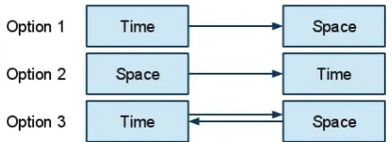
of drought in this study differs from space to time, therefore an integrated drought concept is proposed. From a time se-ries analytical point of view the definition of drought is in-terpreted as an anomaly of low values in the time series of the hydrological variable in a cell. On the other hand, in space anomalies of low values of a hydrological variable can be interpreted as a drought region. Therefore, the possible approaches can be represented as in Fig. 1.

– Option 1: Analysis of drought is performed by identi-fying anomalies determined and characterized by time series statistics (e.g. percentiles). Overall statistical in-formation of the events are grouped and then the spatial analysis is done. This can be done by investigating the overall statistical information of a group of cells, or by spatially smoothing the statistical information.

– Option 2: Analysis of drought regions in one time frame (e.g. particular day, month or year) is performed (no knowledge from past or future time frames is assumed). Regions that have anomalies of water flow or levels are clustered (grouped) and labelled (classified) as drought. This cluster procedure is evaluated at different time frames and matching patterns of the anomalies of the regions are compared.

– Option 3: First the time dimension is considered as in Option 1, however, a second analysis is done per each time step. In evaluating the spatial regions of the drought at each time step and identifying contiguous ar-eas it is possible to visualize drought development. The main objective of these three options is to cover pos-sible approaches to develop drought area analysis. These three options can be reflected in (i) overall cluster of statis-tics, (ii) Non-Contiguous Drought Area (NCDA) analyses, and (iii) the Contiguous Drought Area (CDA) analyses. The latter two methodologies are presented here to investigate hy-drological drought at large scales. The NCDA analysis in this study focuses on the globe as a whole and on some selected large hydro-climatic regions. Additionally, the CDA analy-sis focuses on linked cells that have neighbours with the same conditions (e.g. drought state) and therefore can be clustered and labelled as spatial drought event.

The detailed procedure of the analysis can be divided into four steps as shown in Fig. 2. Although step 3 is not required for the CDA method, it is an important analysis that helps with the overall identification and location of drought. Here-after we present the temporal drought analysis (steps 1 and 2) followed by the NCDA and CDA methods (steps 3 and 4). 2.1 Drought analysis in the time series domain (steps 1

and 2)

To determine droughts from the modelling results the thresh-old level method (Yevjevich, 1967; Hisdal et al., 2004) is applied. With this method, a drought occurs when the

Fig. 1. Diagram of the steps in a temporal and spatial analysis.

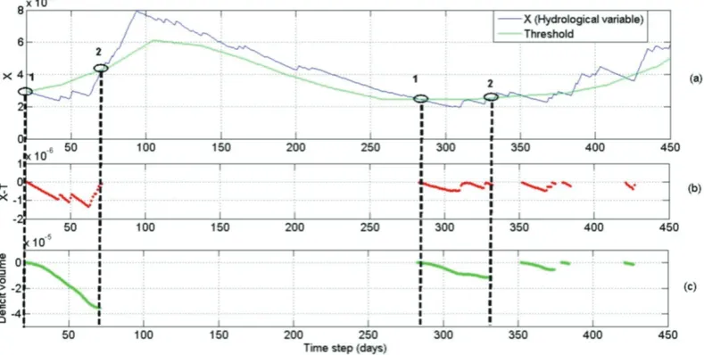
variable of interest (e.g. precipitation, soil moisture, ground-water storage, or discharge) is below a predefined threshold (Fig. 3). The start of a drought event is indicated by the point in time when the variable falls below the threshold and the event continues until the threshold is exceeded again. Hence, each drought event can be characterised by its beginning, end and duration. Other commonly used drought characteristics are: deficit volume, calculated by summing up the differ-ences between actual flow and the threshold level over the drought period, and minimum flow during an event (Hisdal et al., 2004). Both a fixed and a variable (seasonal, monthly, or daily) threshold can be used. In this study, a monthly thresh-old derived from the frequency duration curves of daily data are taken. For cells with a perennial runoff relatively low thresholds in the range from the 70 to 95-percentile can be considered reasonable (e.g. Hisdal et al., 2004; Fleig et al., 2006). In this study the 80-percentile is selected (e.g. Hisdal et al., 2001; Andreadis et al., 2005; Tallaksen et al., 2009; Wong et al., 2011), meaning that subsurface runoff values are exceeded 80 % of the time. Although it is possible to think on more fuzzy bounds for the drought identification of a cell, this is not contemplated in this study. For cells with an inter-mittent or ephemeral runoff having a majority of zero flow, the 80-percentile could easily be zero in one or more months, and hence no drought events would be selected for these months. For these dry regions a higher threshold (low per-centile) can be chosen as proposed by Fleig et al. (2006), or the region can be excluded because drought in streamflow is not so meaningful. The latter has been done in this study, al-though the proposed methodology can handle higher thresh-olds. Dry regions were excluded from the drought analysis when in more than 80 % of the time the simulated runoff is zero. If the percentage of zero flow is lower than 80 %, but the time series presents one single event, in the period 1963– 2001, which appears in arid regions, it is also excluded. The discrete monthly threshold values are smoothed by applying a moving average of 30 days (e.g. van Loon et al., 2010). The smoothed threshold (T) and the hydrological variable are shown in Fig. 3. It is important to highlight that minor droughts are removed. Several methods have been proposed in the literature depending on dynamics of the hydrological variable (e.g. Fleig et al., 2006). The proposed methodol-ogy is flexible and different approaches and values can be used. In this study minor droughts with a duration smaller than 3 days (10 % of a month) are excluded.

2966 G. A. Corzo Perez et al.: Spatio-temporal analysis of hydrological droughts

The detailed procedure of the analysis can be divided into four steps as shown in Fig. 2. Although

step 3 is not required for the CDA method it is an important analysis that helps with the overall

representation of the drought region. Here after we present the temporal drought analysis (steps 1

and 2) followed by the NCDA and CDA methods (steps 3 and 4).

120

Fig. 2. Diagram of temporal and spatial analysis interaction

2.1

Drought analysis in the time series domain (steps 1 and 2)

Fig. 3. Drought characteristics calculated with defined variable threshold: (a) Hydrological variable and

vari-able threshold, (b) daily intensity, (c) event deficit volume. Start and end of the events are named as 1 and

2

To determine droughts from the modelling results the threshold level method (Yevjevich, 1967;

Hisdal et al., 2004) is applied. With this method, a drought occurs when the variable of interest

(e.g. precipitation, soil moisture, groundwater storage, or discharge) is below a predefined threshold

5

Fig. 2. Diagram of temporal and spatial analysis interaction.

Fig. 3. Drought characteristics calculated with variable threshold: (a) Hydrological variable and variable threshold, (b) daily intensity, (c) event deficit volume. Start and end of the events are named as 1 and 2.

From the identification of drought events using the vari-able threshold method we extract the drought characteristics of each cell. The drought characteristics that fit our purpose are the average drought duration, average drought deficit vol-ume and number of events. These drought characteristics are calculated as follows (similar to Sheffield et al., 2009; Tal-laksen et al., 2009).

The drought duration (DD) is determined by the period of time the variable is under the drought threshold. DD is the total drought duration at cellcof a particular event.

ADD =

PN

i=1DD

N (1)

where ADD is the average drought duration at cellc(N is the number of droughts per cell).

The deficit volume (DV) is calculated by accumulating the daily deficit (X−T) as visualized in Fig. 3.Xrepresents the

value of the simulated variable (in this study the subsurface runoff Qsb).

DVi = te

X

t=ts

(Xt −Tt) (2)

where DVi is the deficit volume of the eventi. The initial

and final time steps are represented byts andterespectively. Tt is the threshold per time step.

RADV =

PN i=1DVi

N

,

std(X) (3)

where RADV is the relative average deficit volume at cellc. The division by the standard deviation (std(X)) is imple-mented since in the spatial analyses it is required to compare relative (standardized) and not absolute values.

ADI =

PN i=1DVi

N

,

ADD(X) (4)

where ADI is the Average Drought Intensity per cell.

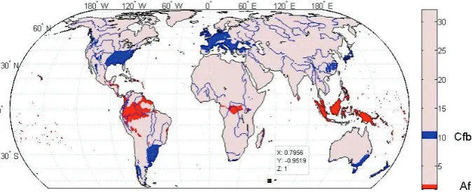
Fig. 4. Selected K¨oppen-Geiger regions used for the NCDA analysis.

2.2 Spatial methodology

The two proposed methodologies, NCDA and CDA can be explained as follows.

2.2.1 Non-contiguous drought areas (NCDA, step 3)

The spatial analysis presented here is based on the occur-rence of an event (binary representation). Therefore, a dis-crete drought stateDs per cell was used. This can be

ex-pressed by a function (Eq. 5). Ds(t ) =

1 ifXt < Tt

0 ifXt ≥ Tt

(5) where the drought state Ds per cell at time step t is

de-termined by the hydrological simulated variableX at each timet.

PDA(t ) = 100/Atot · N

X

c=1

(Ds(t )· A) (6)

where PDA is the percentage of area in drought, at time t and relative toAtot(total land area considered, e.g. the globe,

climatic region, continent). The area at each cellAin this study was calculated according to its projection,Nis number of cells. These equations were applied to global and selected hydro-climatic regions as follows.

– Global spatial analysis of droughts:

the spatial analysis is performed by applying Eqs. (5) and (6) to all cells across the globe at each time step. The result provides an overall assessment of the area in drought (% of global land area) as well as the critical pe-riods (months or years) where this percentage is higher than normal.

– Regional drought spatial analysis (continents or climate regions):

in this study we use both continents and climatic re-gions. The spatial analysis of climatic regions is based on a division of the study space (globe) into regions

that are defined by climate criteria. This is achieved by grouping cells that have similar climate properties. In this study we used the K¨oppen-Geiger classifica-tion (K¨ottek et al., 2006; Peel et al., 2007; Wanders et al., 2010). Wanders et al. (2010) applied the K¨oppen-Geiger classification rules that define each climate to the WATCH Forcing Data (Weedon et al., 2010, 2011) to obtain for each cell a classification. Cells that be-long to the same K¨oppen-Geiger sub-climate were clus-tered. The two regions selected (Af, Cfb) in this study are highlighted in Fig. 4. The “Af” is a tropical rainfor-est climate that is characterized by constant high tem-peratures all the year and all months have average pre-cipitation of at least 60 mm. The clusters are mainly located in the Amazonian and Indonesian regions. The “Cfb” is a humid temperate climate, which can be found in major parts of Europe, Eastern USA, south of South America, Eastern China, Eastern Australia and in some smaller regions.

2.2.2 Contiguous drought areas (CDA, step 4)

The NCDA provides the overall temporal evolution of the area in drought in a predefined region (e.g. globe, conti-nent, hydro-climatic region). However, any of these pre-defined regions are arbitrary reference regions, they might separate spatially-continuous drought events (except for the case of the globe as reference region). Contiguous areas of drought (CDA) reflect spatial drought patterns composed by linked neighbours in a state of drought, classified here as spatial drought event. The binary representation created with the drought states (Eq. 5), from the time series analysis, allows for the application of pattern recognition techniques that group different cells based on the characteristics from their neighbours. This in general can be described as a clus-tering based on its neighbour conditions (e.g. connectivity). For more reference on similar type of approaches please re-fer to Sheffield et al. (2009) who identified drought events in time and space using another clustering algorithm, and An-dreadis et al. (2005) and Zaidman et al. (2002) who presented

2968 G. A. Corzo Perez et al.: Spatio-temporal analysis of hydrological droughts severity-area-duration curves with a partitioning, smoothing

and filtering process for the clustering in the spatial dimen-sion. The method used within this study can be described as follows.

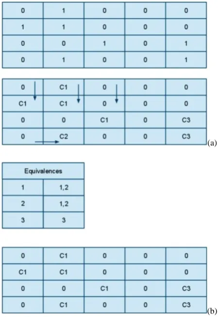
1. Scan all cells of the data first by column then by row (Fig. 5).

2. Evaluate the state of the 8 (or 4 neighbours) and assign a preliminary class (spatial drought label) to the cell. Assignation is done as follows.

– If actual position of the cell is in drought then look for a neighbour in drought.

– If a neighbour is in drought and has a label (class) then change the label of the actual cell to the label of the neighbour.

– If there is more than one label between the neigh-bours assign the lowest one and store the equiva-lence in the equivaequiva-lence table.

– Else assign a new label number.

3. Resolve the table of equivalence classes leaving linked classes as one class.

4. Make a second iteration from column cells then row and relabel based on the resolved equivalence classes. The algorithm can be applied using different numbers of neighbours, for the present study we used 8 neighbours (Dil-lencourt et al., 1992).

The number of spatial events is reduced applying similar criteria as other previous studies (Sheffield et al., 2009; Tal-laksen et al., 2009). An areal threshold is defined with a min-imum area required to have a spatial event (in this study the areal threshold was 2 cells, approx. a minimum of 5000 km2). Therefore in this study we excluded spatial events with an area below or equal to 2 connected cells in drought. This rather low areal threshold still allows for identifying spatial droughts in small units of the selected K¨oppen-Geiger re-gions.

3 WaterGAP model simulation

The gridded outcome from the global hydrological model WaterGAP was used in this study to further develop NCDA and CDA approaches for hydrological drought and to illus-trate these across large scales. The global hydrological mod-eling system WaterGAP has been widely used on exploring the distribution and availability of water resources. It has been tested against river flow data and has shown to be a pow-erful tool to simulate the global water cycle. WaterGAP com-bines a global hydrological model (Alcamo et al., 2003; D¨oll et al., 2003) with several global water use models (Fl¨orke et al., 2010; Fl¨orke and Alcamo, 2004; Alcamo et al., 2003;

(a)

(b)

Fig. 5. Example of the steps for linking neighbours in a drought

cluster (for detailed explanations see Sect. 2.2.2). (a) Step 1 and

(b) Step 2.

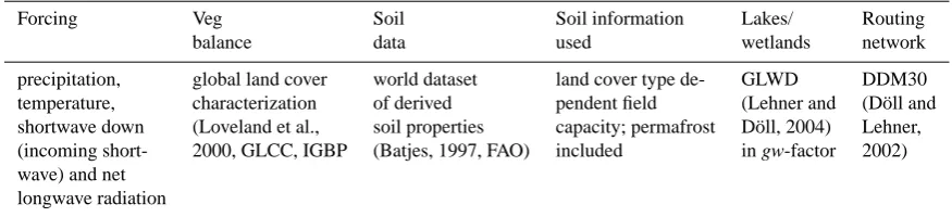
D¨oll and Siebert, 2002). The WaterGAP Global Hydrology Model calculates surface and subsurface runoff, groundwa-ter recharge and river discharge at a spatial resolution of 0.5◦ and is well applicable for global assessments related to wa-ter security, food security and freshwawa-ter ecosystems. To simulate the terrestrial water cycle spatially distributed phys-iographic information about elevation, slope, hydrogeology, land cover and soil properties, as well as location and ex-tent of lakes, wetlands, and reservoirs is used. In addition climate data like precipitation, temperature and different ra-diation terms need to be specified (see Table 1). Optionally, water required for consumptive water use can be subtracted from surface waters. In this study only naturalized model simulations (i.e. without taking water management and water uses into account) were utilized (e.g. Haddeland et al., 2011). As a hydrological variable the simulated daily, gridded sub-surface runoff was selected, which represents the groundwa-ter component of the hydrological drought. So far, Wagroundwa-ter- Water-GAP has not been calibrated at a daily timescale, neverthe-less we expect this to have no significant effect on the drought analysis, because daily subsurface runoff appears to have no high intra-monthly flow variability for most of the cells. The

Table 1. WaterGAP model setup information.

Forcing Veg Soil Soil information Lakes/ Routing

balance data used wetlands network

precipitation, global land cover world dataset land cover type de- GLWD DDM30 temperature, characterization of derived pendent field (Lehner and (D¨oll and shortwave down (Loveland et al., soil properties capacity; permafrost D¨oll, 2004) Lehner, (incoming short- 2000, GLCC, IGBP (Batjes, 1997, FAO) included in gw-factor 2002) wave) and net

longwave radiation

spatial resolution of the model results for each hydrological variable is 0.5◦latitude by longitude, covering land areas de-fined by the CRU (Climate Research Unit of the University of East Anglia) land mask. Although WaterGAP was run from 1958 to 2001, only outcome from 1963 onwards is used since the model requires a warming period (e.g. 1958–1962). Only land point cells from the CRU mask were considered in this analysis (total land area is 146.7 million km2; distributed over 67 420 cells). The total land area above the equator rep-resents around 78 % of the total land area.

We used the WATCH forcing data (Weedon et al., 2010, 2011) to force the WaterGAP model. The WATCH forcing variables are taken from the ERA-40 reanalysis product of the European Centre for Medium Range Weather Forecasting (ECMWF) as described by Uppala et al. (2005), and are in-terpolated to 0.5◦spatial resolution, including elevation cor-rections as well as different methods for bias and/or under catch corrections. For detailed information on the forcing variables see Weedon et al. (2010, 2011).

4 Results

The development of the CDA and NCDA methodologies was evaluated for two different time periods. A long record of 38 years of daily time steps starting in 1963 was used for the NCDA. Part of this record, starting from 1976 (25 years) was used for the CDA. The period for the CDA was se-lected based on the highest number of droughts found in the run of the NCDA analysis. The CDA computational time is rather high and therefore this shorter period was beneficial. Both for the NCDA and the CDA, the same monthly variable thresholds were used for each cell, which were derived from the time series that cover the whole period of 38 years. 4.1 Time series results

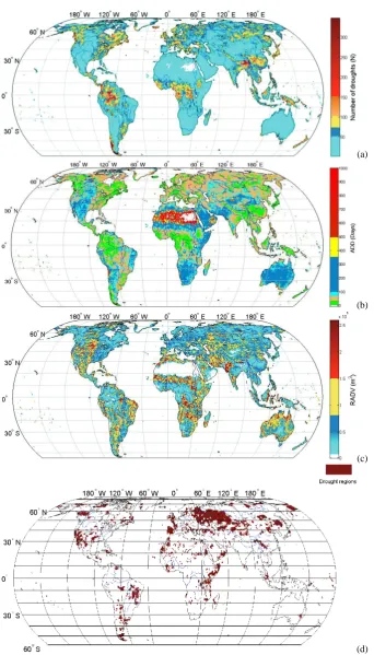
Figure 6a–c shows global maps with drought characteris-tics. Some regions show up as white areas (Fig. 6a) mean-ing that in 80 % of the time the simulated subsurface is zero (e.g. Sahara desert in Africa). On the other hand it is possi-ble to see regions with a low number of spatial events that

are located on non-polar arid lands like, Sonora and Chi-huahua, in Mexico and Atacama, in Peru and Chile. This drought behaviour of semi-arid and arid land is a clear out-come of the threshold method, which evaluates the events as a measure of the time when the flow is below a predefined low value. Climatic regions, where rainfall is erratic and low runoff is present for long periods of time, will have less num-ber of events. Figure 6b shows a contrasting picture to what we saw in Fig. 6a. According to the definition low num-bers of droughts go along with high average durations and the other way around. The Sahara desert and other extremely arid lands have drought durations of more than 2 years (500– 1000 days), and arid lands (see Meigs, 1973, for a detailed definition) durations of around 0.5–1 year (100–300 days).

The distribution of the relative average deficit volume (RADV) is mixed and only spotted values can be seen in north west and middle USA, where high RADV seems to have some relation with average duration of 100 to 300 days (Fig. 6c). This pattern also occurs in the north eastern region of Brazil near the state of Maranhao.

Figure 6d shows, as an example, the drought pattern at the beginning of 1976. The drought characteristics presented in Fig. 6 show the importance of further exploring global dis-tribution of drought characteristics with the NCDA and CDA methodology presented in this study. The NCDA global re-sults can be visualized at each time step (Fig. 6d) to fur-ther support the analysis of the global drought characteristics (Fig. 6a–c).

4.2 Global results (NCDA)

The Percentage of Drought Area (PDA) for each time step is explored using Eq. (6). Figure 7a shows the evolution of the PDA of the whole globe for the period between 1963 till 2000. From the yearly time series it is possible to derive the bound of maximum and minimum PDA, 30 % and 12 % respectively. The maximum PDA appears at the time series for the year 1992.

The color-coded map in Fig. 7b is built using the time se-ries of PDA and a color representation for each percentage. The color-coded table shows some persistence among the years at the global scale (e.g. 1980s). Furthermore, Fig. 7b

2970 G. A. Corzo Perez et al.: Spatio-temporal analysis of hydrological droughts

(a)

(b)

(c)

(d)

Fig. 6. Hydrological drought characteristics derived from the subsurface runoff simulated with the WaterGAP model. (a) Total number of

drought events, (b) average drought duration, (c) relative average deficit volume and (d) spatial distribution of drought events for 13 Jan-uary 1976.

(a)

(a) Time series of area in drought (percentage of the globe)

(b) Color-coded table of area in drought (as percentage of the globe area)

Fig. 7.Results of the NCDA analysis over the globe for the period 1963-2001.

29

(b)

Fig. 7. Results of the NCDA analysis over the globe for the period 1963–2001. (a) Time series of area in drought (percentage of the globe)

and (b) color-coded table of area in drought (as percentage of the globe area).

Fig. 8. Development of the PDA in six selected major K¨oppen-Geiger hydro-climatic regions over the years 1991 to 1993 (red line is 1992).

shows a low percentage of area in drought between the be-ginning of 1974 to the middle of the year 1976, as well as from the beginning of 1978 to first months of 1980. On the other hand, higher percentages can be seen from April till July 1982 and from February till August 1992. The high-est percentage in 1992, seems to be not clearly preceded by other dry years. Other high PDAs can be seen in 1998 where the beginning of the high percentage appears at the end of 1997. Most of the historical high PDAs occur between cal-endar day 75 to 150 (April–May). This seems to happen in spring and the early summer for the Northern Hemisphere

and transition summer–autumn in the Southern Hemisphere. The last 130 days of most years, the time series seems to be stable and no important variations can be seen from the beginning (day 230) to the end (day 360).

As mentioned above, the global PDAs show a seasonal behaviour, in particular between days 75 and 150, which seems to be associated with the transition of seasons, of-ten together with high climate variability. To explore such phenomena, the PDAs for six major K¨oppen-Geiger hydro-climatic regions (Fig. 8) over the years 1991–1993 were plot-ted. The selected regions include a wide range of climates,

2972 G. A. Corzo Perez et al.: Spatio-temporal analysis of hydrological droughts

(a) Areas with tropical rainforest climate (Af)

(b) Areas with maritime, temperate climate (Cfb)

Fig. 9. Daily time series of percentage of area in drought for each year in the period 1963 to 2001 in Af and

Cfb climates.

31

(a)

(a) Areas with tropical rainforest climate (Af)

(b) Areas with maritime, temperate climate (Cfb)

Fig. 9. Daily time series of percentage of area in drought for each year in the period 1963 to 2001 in Af and

Cfb climates.

31

(b)

Fig. 9. Daily time series of percentage of area in drought for each year in the period 1963 to 2001 in Af and Cfb climates. (a) Areas with

tropical rainforest climate (Af) and (b) Areas with maritime, temperate climate (Cfb).

i.e. warm equatorial with dry winter (Aw) or fully humid (Af), arid hot desert (BWh), temperate with warm summer (Cfb), snow-affected with a warm summer (Dfb) or cool summer with cold winter (Dfc). The selected hydro-climatic regions cover about 35 % of the land surface of the globe, implying that these have a substantial influence on the global PDAs (Fig. 7a). Although, there is a clear variability in the lower frequency components of the time series the high fre-quency components dominate. Three climates have a clear seasonality (Aw, Dfb, Dfc). The Dfb climate has a period-ical high PDA around day 90 of each year, when the cold season with snow enters the warm summer (Fig. 8e). The Dfc climate has two PDA peaks around days 90–120, which reflect the transition from the cold winter with snow into the cool summer (Fig. 8f). The Aw climate has less pro-nounced higher PDAs around day 150, which seem to be linked to the start of the monsoon (Fig. 8b). The climates with a clear seasonality have a sharp rise in the runoff either due to snowmelt or onset of the monsoon. Late snowmelt or arrival of the monsoon, which will not occur synchronously in the spatially-distributed units of a hydro-climatic region over the globe, leads to drought (anomaly), which in most year is short lived because the delayed snowmelt or monsoon will stop the drought (e.g. van Loon et al., 2011). Clearly, the definition of the drought through the daily smoothed monthly thresholds (Sect. 2.1) influences the occurrence of anomalies. Drought anomalies clearly linked to a particu-lar time of the year (i.e. day 90–150) because of seasonal climates cause regular patterns in the global PDAs. These patterns need to be superimposed on the patterns of other climates. For example, the Cfb climate has irregular peaks at the end of the winter (e.g. 1992/1993), which likely co-incide with low-rainfall winters (Fig. 8c). The fully humid equatorial climate (Af) and the hot desert climate (BWh) have in common that below average rainfall is not linked to seasons, which gives very unpredictable anomalies in runoff (Figs. 8a and d). The combination of more regular anomalies

in seasonal climates (e.g. Aw, Dfb, Dfc) and rather unpre-dictable timing of anomalies in other climates (e.g. Af, BWh) results in the composite pattern shown in Fig. 7b. Further-more, the unequal distribution of the snow-affected climates (e.g. Dfb, Dfc) over the globe, which predominantly occur in the Northern Hemisphere, cause patterns that show up only in the first part of the year (days: 75–150) and not in the sec-ond part.

4.3 K¨oppen-Geiger hydro-climatic regions (NCDA)

Based on the previous analysis the regions which we call un-predictable behaviour are the Af and the Cfb climates. Per-centages of drought areas for the whole period (1963–2001) were calculated for these two hydro-climatic regions to in-vestigate the spatial differences in the areal coverage across the world.

Figure 9a shows the 38 annual series of the PDA for the clusters with a Af climate (Fig. 4). The PDA values are higher than in the overall analysis for the globe (Fig. 7b), reaching a value of 62 % at the beginning of 1998 and the end of 1997. This is a region that is well known for its rich-ness in water resources on average, nevertheless, it appears to have a high number of anomalies in its low runoff, which can be explained by the rather large inter annual variability. Aside of this, in the year 1992 the most severe PDA over a whole year is shown.

For the second climate regime (Cfb, Fig. 4), the highest PDA is 36 % (Fig. 9b). In this hydro-climatic region, 1992 seems not to have a high area in drought. The year 1976 has the highest PDA for the Cfb region. In the discussion section, the above-mentioned years with high PDAs will be compared with some documented events.

(a) Drought clusters for the 10th of January 1976 (around 800 colors, each color represent a cluster

50 100 150 200 250 300 350

1976 1980 1985 1990 1995 2000

Day

Year

Numder of drought events (clusters)

550 600 650 700 750 800

(b) Color-coded table of the number of drought clusters on the whole Earth

Fig. 10.

Results of the CDA method applied for the analysis of number of drought clusters.

(a) Drought clusters for the 10th of January 1976 (around 800 colors, each color represent a cluster

50 100 150 200 250 300 350 1976

1980 1985 1990 1995 2000

Day

Year

Numder of drought events (clusters)

550 600 650 700 750 800

(b) Color-coded table of the number of drought clusters on the whole Earth

Fig. 10.Results of the CDA method applied for the analysis of number of drought clusters.

32

(b)

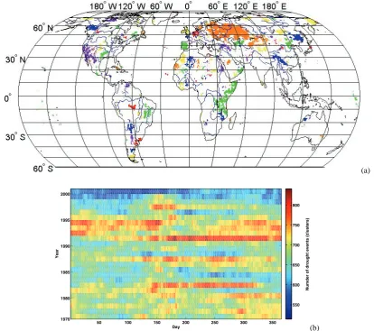
Fig. 10. Results of the CDA method applied for the analysis of number of drought clusters. (a) Drought clusters for 10 January 1976 (around

800 colors, each color represent a cluster and (b) color-coded table of the number of drought clusters on the whole Earth.

4.4 Spatial drought events (CDA)

In contrast to the NCDA presented in the previous sections, the contiguous approach (CDA) focuses on linking neigh-bouring drought states. Connected cells in drought (Ds) can

be interpreted as a spatial drought event. Each spatial drought event (Sect. 2.2.2) is unique for a particular time step, and can be analysed further by exploring its spatial properties. Fig-ure 10a shows, as an example, the results of a clustering anal-ysis for 10 January 1976. For this date more than 800 spatial drought events were found across the globe. To explore the temporal evolution of the number of spatial drought events a color-coded table of 25 years with the number of clus-ters found on each day was plotted (Fig. 10b). The figure shows similar patterns as the NCDA. The minimum number of spatial events was around 400 and therefore the scale of the color-coded bar starts at 500, which means that events with a rather low number of spatial clusters are excluded. The year 1992 stands out as in the NCDA as the most critical

year. Other extreme events, like 1982, 1987 and 1993 also show up in this graphical presentation. This illustrates that the number of spatial drought events seems to be congruent with the global area in drought.

Figure 10a illustrates that the distribution of the spa-tial drought events can follow regions that are not clearly bounded by hydro-climatic classifications. Spatial drought events can be identified inside climatic or regional (e.g. con-tinents) boundaries or its areas can be in multiple hydro-climatic regions at the same time. This means that for de-tailed analysis of spatial events it is important to have un-bounded regions to avoid separation of spatial events.

The main advantages of the CDA is the possibility to iden-tify: (i) the area of a particular spatial event (number of cells or area), and (ii) location (geo-referenced). This can be done for a specific time step as demonstrated in Fig. 10a. Addi-tionally, in a temporal study it also requires monitoring the evolution of spatial drought events for (long) time series (e.g. Andreadis et al., 2005; Lloyd-Hughes, 2010), as well as to

2974 G. A. Corzo Perez et al.: Spatio-temporal analysis of hydrological droughts

(a) Maximum area of the spatial drought event (in cells)

(b) Location of the maximum spatial drought event and number of days

Fig. 11.Occurrence and duration of the maximum spatial drought events for the period 1976–2000.

33

(a)

(a) Maximum area of the spatial drought event (in cells)

(b) Location of the maximum spatial drought event and number of days

Fig. 11.Occurrence and duration of the maximum spatial drought events for the period 1976–2000.

33

(b)

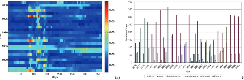
Fig. 11. Occurrence and duration of the maximum spatial drought events for the period 1976–2000. (a) Maximum area of the spatial drought

event (in cells) and (b) location of the maximum spatial drought event and number of days.

summarize statistically their information. In this study we monitor the maximum area of a spatial drought event and the duration (i.e. number of days in a calendar year) that it oc-curs somewhere in the world. This was done to keep track of the change in Maximum Spatial Drought Event (MSDE) in terms of its size and relative location at each time step. Figure 11a shows a color-coded table with the timing and the magnitude of the MSDEs for each day within the 25 year record contemplated in this part of the study. MSDEs of above 5000 cells (about 7.5 % of the global land area) ap-pear only around 6 times for a maximum of 30 days. Fur-thermore, we see, although weaker, similar patterns around days 75–150 as for the global area in drought (Fig. 7b). Be-cause of the congruence of area in drought and number of spatial events it is possible that seasonal climates cause these patterns (Sect. 4.2).

The relative location of MSDE is an important indicator of changes in global drought. For this, the occurrence of the MSDE in a continent, is determined by the location of its ge-ometrical centroid. This analysis for continents does not re-late to a predefined region, and although a MSDE is counted for a particular continent, it may extend over the continents border. Figure 11b shows how many days the centroid of the MSDE occurs in the different continents. For instance, in 1999 the maximum event was found in Asia for over 300 days and for about 50 days in North America. The maxi-mum area seems to be located predominantly in Asia. Africa has continuous records with events from 1983 till 1985. Ex-ceptional cases in Europe can be highlighted like 1976 which has a high number of days that the maximum spatial drought event occur there (over 60 days).

5 Discussion

In this study the analysis of spatial and temporal droughts from a global hydrological model has been developed using overall statistics as well as the CDA and NCDA methodolo-gies. A number of remarks can help on the understanding of the benefits and weakness of the methodologies. For the characterization of spatial drought events a unique formula-tion is required, since convenformula-tional averaging of spatial re-gions might not really represent relevant characteristics of the drought. The duration of a spatial event could be defined by the average, longest or shortest duration of the cluster of connected neighbourhood cells. However, to determine the deficit volume of a particular spatial event, it might not be accurate to add straightforwardly deficits. Instead, a weight-ing of normalized volumes can be calculated as an alterna-tive. Moreover, the spatial extent of the events is changing in time (e.g. Andreadis et al., 2005; Lloyd-Hughes, 2010), as well as its centroid. Therefore a morphological and dynamic analysis needs to be included in the CDA method presented in this paper. In this sense, this paper did not cover the de-velopment of drought characteristics of these spatial events (e.g. dynamics of representative drought duration or deficit volume of a cluster).

The duration and deficit volume severity of a spatial drought event, at a particular time, is relevant information for drought management. This is commonly approached us-ing severity-area-duration (SAD) curves (e.g. Shefield et al., 2009), however, the approximation of this method is limited by the spatial interpolation used on the overall information. Therefore, the CDA could be a complementary methodology that provides a step by step spatial analysis.

Drought characteristics both for the NCDA and CDA methodologies are affected by the definition of drought, es-pecially the choice of threshold, the approach to remove mi-nor droughts (Hisdal et al., 2004; Fleig et al., 2006) and the

methods to deal with zero flows. Smoothing of the hydro-graph by applying ak-day moving average (Fleig et al., 2006; Wong et al., 2011) and implementing multiple threshold are commonly considered for the temporal analysis. A step for-ward in the analysis of spatial drought events is to explore the temporal and spatial sensitivity of applying different areal thresholds (in this study two cells). If higher areal thresh-olds are applied (e.g. Sheffield et al., 2009) only large events will be identified, which implicitly means exclusion of small (spotted) regions, i.e. small units of K¨oppen-Geiger climates. Another important feature is that the CDA algorithm used has a two dimensional neighbouring scheme (latitude and longi-tude). This scheme only includes regions with 8 contiguous cells in drought, but by increasing the range of neighbours to, for instance, 24 cells it will reduce the sensitivity of the areal threshold by only identifying larger spatial events. Another spatial criterion that requires investigation is the number of cells not in drought that should separate two adjacent spa-tial drought events. In this study, a single line of cells not in drought, may break one large event into two separate events. Some of the NCDA and CDA results obtained in this study with a single global hydrological model (WaterGAP) have interesting similarities to reported historical events. The ma-jor drought area obtained for the year 1992 correspond to the El Ni˜no Northern Oscillation (ENSO) year. The years 1997 and 1998, which correspond also to the ENSO phenomena (clearly present in Indonesia and South America, Aceituno, 1988; Chokkalingam et al., 2005), show to have a high per-centage of drought area in the NCDA (Af region) and a high number of spatial drought events in the CDA.

The European drought in 1976 is clearly elucidated in the CDA and NCDA, and its durations seem to match with previ-ous studies (Hisdal et al., 2004; Hannaford et al., 2010). The Cfb region has an important component in Europe (Fig. 4) and in many studies the 1976 European drought has been studied due to the high economic impact (Stahl, 2001). Al-though in our study, with the CDA, the maximum spatial event in 1976 is not as high as it was expected (Fig. 9a), that year had a long period of time with the maximum drought event in the globe. In 1991–1992 there was a prolonged drought over the Iberia peninsula (Hisdal et al., 2004). The CDA shows a maximum drought event centroid in a long period of time over US, having a link to the severe ex-treme drought in over half of the country during 1987–1989 (Fig. 11b). This drought was the subject of national head-lines when it resulted in the extensive fires in Yellowstone National Park in 1988 (Sheffield et al., 2009; Andreadis et al., 2005; Shukla and Wood, 2008). It is documented that Africa suffered from droughts in the last quarter of the twentieth century (Prospero and Nees, 1986). The years 1984 and 1985 show to have the largest spatial drought event in Africa, which is highly associated to the drought and famine in East Africa. Ethiopia, usually considered the breadbasket of East-ern Africa, was hit by a extreme drought in the early 1980’s. A dry year in 1981 resulted in low crop yields. This period

can be clearly identified in the Fig. 11b. Application of the NCDA to hydro-climatic regions that are affected by phe-nomena like the ENSO can be useful to test the approach (with single or multi-model), since with the global infor-mation (Fig. 6) it is not possible to capture these phenom-ena. Other regional distributions of the earth, can help on model inter-comparison, since models might perform better or worse according to different hydro-climatic regions.

6 Conclusions

In this study, two concepts of spatio-temporal analysis of large scale drought have been further developed. These con-cepts are the non-contiguous drought areas (NCDA) and the contiguous drought areas (CDA) approach. The NCDA anal-ysis for the globe and pre-defined hydro-climatic regions builds upon principles used at the river basin scale as pro-posed by Tallaksen et al. (2009). In a similar way, tempo-ral analysis with a variable threshold followed by spatial as-sessment was presented (Fig. 6). The CDA presented here is based on the use of an objective and automatic grouping of spatial drought events. This objective determination of spa-tial drought events uses pattern recognition on binary rep-resentations of drought and connected labelling algorithms. The NCDA and CDA analyses used subsurface flow values from the WaterGAP global hydrological model (second part 20th century).

The NCDA is useful for assessing overall spatial drought information at global and regional scales, while the CDA showed specific extreme areas that are unbounded by pre-defined regions. NCDA results seem to capture important events that might appear to be connected to relevant histori-cal events. The ENSO phenomena and the droughts in Eu-rope (1976 and 1992) show up in different ways in outcome from both methods. With the NCDA a high percentage of area in drought was identified and with the CDA a high area spatial events was found.

The centroid of the maximum spatial drought event in the CDA analysis was used as a measure of extreme events in the different continents (Fig. 11b). Its duration is assumed to reflect drought persistence in a continent. Both the NCDA and CDA investigate drought patterns (Figs. 9a and 11b), which suggest that global drought has its maximum extent in a particular season (March–May). Seasonal climates char-acterized by irregular snow melt (e.g. Dfb and Dfc climates) or Monsoon are the reason for these rather short anoma-lies. Dominant occurrence of these climates in the Northern Hemisphere contributes to these seasonal drought patterns.

The CDA shows to be able to identify spatial drought events and at the same time it is possible to follow critical (the most extended) events along time as illustrated for the continents. However, important characteristics, like deficit volume and duration of spatial events, require an analysis to be able to reach indices that characterize their drought

2976 G. A. Corzo Perez et al.: Spatio-temporal analysis of hydrological droughts severity. Aside of this, morphological changes and

track-ing of spatial drought events seems to be the way forward to further explore spatial events and see how well global hy-drological models capture historical events. Although the NCDA and CDA methodologies presented here used subsur-face flow, these are flexible and can be applied to similar vari-ables and other drought identification approaches, e.g. the Sequent Peak Algorithm (Hisdal et al., 2004). Further re-search steps are being taken towards the sensitivity of thresh-olds (e.g. introduction of multiple threshthresh-olds), the removal of minor droughts and the treatment of cells with high number of zero flow in a multi-model intercomparison context.

The two methodologies presented here can capture the main spatial temporal characteristics of large scale droughts. The results can help to: (i) understand drought genera-tion as response to climate drivers and physical river basin structures, including possible world-wide synchronicity, and (ii) used to asses the impact of global change on drought (21st Century drought).

Acknowledgement. This research was undertaken as part of the

European Union (FP6) funded Integrated Project Water and Global Change (WATCH, contract 036946). The research is part of the programme of the Wageningen Institute for Environment and Climate Research (WIMEK-SENSE). The study contributes to the UNESCO IHP-VII programme (Cross-cutting programme FRIEND and Theme 1 Adapting to the impacts of global changes on river basins and aquifer systems).

Edited by: F. Pappenberger

References

Aceituno, P.: On the functioning of the Southern Oscillation in the South American sector, Part I: Surf. climate, Mon. Weather Rev., 116, 505–524, 1988.

Alcamo, J., D¨oll, P., Henrichs, T., Kaspar, F., Lehner, B., R¨osch, T., and Siebert, S.: Development and testing of the WaterGAP 2 global model of water use and availability/D´eveloppement et ´evaluation du mod`ele global WaterGAP 2 d’utilisation et de disponibilit´e de l’eau, Hydrolog. Sci. J., 48, 317–337, 2003. Andreadis, K., Clark, E., Wood, A., Hamlet, A., and

Letten-maier, D.: Twentieth-century drought in the conterminous United States, J. Hydrometeorol., 6, 985–1001, doi:10.1175/JHM450.1, 2005.

Bates, B., Kundzewicz, Z., Wu, S., and Palutikof, J.: Climate Change and Water: Technical Paper of the Intergovernmental Panel on Climate Change, Intergovernmental Panel on Climate Change, 2008.

Batjes, N.: A world dataset of derived soil properties by FAO-UNESCO soil unit for global modelling, Soil Use Manage., 13, 9–16, 1997.

Chokkalingam, U., Kurniawan, I., and Ruchiat, Y.: Fire, liveli-hoods, and environmental change in the middle Mahakam peat-lands, East Kalimantan, Ecol. Soc., 10, 26, 2005.

Dillencourt, M. B., Samet, H., and Tamminen, M.: A general ap-proach to connected-component labeling for arbitrary image rep-resentations, J. ACM, 39, 253–280, doi:10.1145/128749.128750, 1992.

D¨oll, P. and Lehner, B.: Validation of a new global 30-min drainage direction map, J. Hydrol., 258, 214–231, 2002.

D¨oll, P. and Siebert, S.: Global modeling of irrigation water requirements, Water Resour. Res., 38(4), 8.1–8.10, doi:10.1029/2001WR000355, 2002.

D¨oll, P., Kaspar, F., and Alcamo, J.: Computation of global water availability and water use at the scale of large drainage basins, Math. Geol., 4, 111–118, 1999.

D¨oll, P., Kaspar, F., and Lehner, B.: A global hydrological model for deriving water availability indicators: model tuning and vali-dation, J. Hydrol., 270, 105–134, 2003.

Douglas, E., Vogel, R., and Kroll, C.: Trends in floods and low flows in the United States: impact of spatial correlation, J. Hydrol., 240, 90–105, 2000.

EC: Communication Addressing the challenge of wa-ter scarcity and droughts in the European Union, http://ec.europa.eu/environment/water/quantity/scarcity en.htm, last access: 30 September 2010, European Commission, COM 2007, 414 final, Brussels, 2007.

Fleig, A. K., Tallaksen, L. M., Hisdal, H., and Demuth, S.: A global evaluation of streamflow drought characteristics, Hydrol. Earth Syst. Sci., 10, 535–552, doi:10.5194/hess-10-535-2006, 2006. Fleig, A. K., Tallaksen, L. M., Hisdal, H., and Hannah, D. M.:

Re-gional hydrological drought in north-western Europe: linking a new Regional Drought Area Index with weather types, Hydrol. Process., 25, 1163-1179, doi:10.1002/hyp.7644, 2010.

Fl¨orke, M. and Alcamo, J.: European outlook on water use, Center for Environmental Systems Research, University of Kassel, Final Report, EEA/RNC/03/007, 2004.

Fl¨orke, M., B¨arlund, I., and Teichert, E.: Future changes of fresh-water needs in European power plants, Manage. Environ. Qual., 22, 89–104, doi:10.1108/14777831111098507, 2010.

Haddeland, I., Clark, D., Franssen, W., Ludwig, F., Voss, F., Ar-nell, N., Bertrand, N., Best, M., Folwell, S., Gerten, D., Gomes, S., Gosling, S. N., Hagemann, S., Hanasaki, N., Harding, R., Heinke, J., Kabat, P., Koirala, S., Oki, T., Polcher, J., Stacke, T., Viterbo, P., Weedon, G. P., and Yeh, P.: Multi-model estimate of the global water balance: setup and first results, J. Hydrometeo-rol., doi:10.1175/2011JHM1324.1, in press, 2011.

Hannaford, J., Lloyd-Hughes, B., Keef, C., Parry, S., and Prud-homme, C.: Examining the large scale spatial coherence of European drought using regional indicators of precipita-tion and streamflow deficit, Hydrol. Process., 25, 1146-1162, doi:10.1002/hyp.7725, 2010.

Hannah, D. M., Demuth, S., van Lanen, H. A. J., Looser, U., Prud-homme, C., Rees, R., Stahl, K., and Tallaksen, L. M.: large scale river flow archives: importance, current status and future needs, Hydrol. Process., doi:10.1002/hyp.7794, in press, 2010. Heim Jr., R.: A review of twentieth-century drought indices used in

the United States, B. Am. Meteorol. Soc., 83, 1149–1165, 2002. Hisdal, H., Stahl, K., Tallaksen, L. M., and Demuth, S.: Have streamflow droughts in Europe become more severe or frequent?, Int. J. Climatol., 21, 317–333, 2001.

Hisdal, H., Stahl, K., Tallaksen, L. M.: Estimation of regional mete-orological and hydrological drought characteristics: a case study for Denmark, J. Hydrol., 281, 230–247, 2003.

Hisdal, H., Tallaksen, L., Clausen, B., Peters, E., and Gustard, A.: Hydrological drought characteristics, Hydrological drought, Pro-cesses and estimation methods for streamflow and groundwater, in: Developments in Water Science, 48, Elsevier Science B. V., 139–198, 2004.

K¨ottek, M., Grieser, J., Beck, C., Rudolf, B., and Rubel, F.: World map of the K¨oppen-Geiger climate classification updated, Mete-orol. Z., 15, 259–263, 2006.

Lehner, B. and D¨oll, P.: Development and validation of a global database of lakes, reservoirs and wetlands, J. Hydrol., 296, 1–22, 2004.

Liang, X., Lettenmaier, D., Wood, E., and Burges, S.: A simple hy-drologically based model of land surface water and energy fluxes for general circulation models, J. Geophys. Res., 99, 14415– 14428, 1994.

Lins, H. and Slack, J.: Streamflow trends in the United States, Geo-phys. Res. Lett., 26, 227–230, 1999.

Lloyd-Hughes, B.: A spatio-temporal structure-based approach to drought characterisation. Int. J. Climatol., doi:10.1002/joc.2280, in press, 2010.

Loveland, T., Reed, B., Brown, J., Ohlen, D., Zhu, Z., Yang, L., and Merchant, J.: Development of a global land cover characteristics database and IGBP DISCover from 1 km AVHRR data, Int. J. Remote Sens., 21, 1303–1330, 2000.

Meigs P.: World distribution of coastal deserts, Coastal deserts: their natural and human environment, University of Arizona Press, Tucson, 438, 3–13, 1973.

Milly, P., Dunne, K., and Vecchia, A.: Global pattern of trends in streamflow and water availability in a changing climate, Nature, 438, 347–350, 2005.

Peel, M. C., Finlayson, B. L., and McMahon, T. A.: Updated world map of the K¨oppen-Geiger climate classification, Hy-drol. Earth Syst. Sci., 11, 1633–1644, doi:10.5194/hess-11-1633-2007, 2007.

Peters, E., Bier, G., van Lanen, H. A. J., and Torfs, P. J. J. F.: Propa-gation and spatial distribution of drought in a groundwater catch-ment, J. Hydrol., 321, 257–275, 2006.

Prospero, J. and Nees, R.: Impact of the North African drought and El Nino on mineral dust in the Barbados trade winds, Nature, 320, 735–738, 1986.

Sheffield, J. and Wood, E.: Global trends and variability in soil moisture and drought characteristics, 1950–2000, from observation-driven simulations of the terrestrial hydrologic cy-cle, J. Climate, 21, 432–458, 2008.

Sheffield, J., Andreadis, K., Wood, E., and Lettenmaier, D.: Global and continental drought in the second half of the twentieth cen-tury: Severity-area-duration analysis and temporal variability of large scale events, J. Climate, 22, 1962–1981, 2009.

Shukla, S. and Wood, A.: Use of a standardized runoff index for characterizing hydrologic drought, Geophys. Res. Lett., 35, L02405, doi:10.1029/2007GL032487, 2008.

Stahl, K.: PhD thesis: Hydrological drought – a study across Eu-rope, Ph.D. thesis, Universit¨atsbibliothek Freiburg, Germany, 2001.

Stahl, K., Hisdal, H., Hannaford, J., Tallaksen, L. M., van Lanen, H. A. J., Sauquet, E., Demuth, S., Fendekova, M., and J´odar, J.: Streamflow trends in Europe: evidence from a dataset of near-natural catchments, Hydrol. Earth Syst. Sci., 14, 2367–2382, doi:10.5194/hess-14-2367-2010, 2010.

Tallaksen, L. M. and van Lanen, H. A. J.: Hydrological drought: processes and estimation methods for streamflow and groundwa-ter, Developments in Water Science, 48, Elsevier Science B. V., 2004.

Tallaksen, L. M., Hisdal, H., and van Lanen, H. A. J.: Space-time modelling of catchment scale drought characteristics, J. Hydrol., 375, 363–372, 2009.

United Nations International Strategy for Disaster Reduction Secretariat (UNISDR), ISBN/ISSN: 9789211320282, Geneva, Switzerland, p.207, 2009.

Uppala, S., Kallberg, P., Simmons, A., Andrae, U., Bechtold, V., Fiorino, M., Gibson, J., Haseler, J., Hernandez, A., Kelly, G. A., Li, X., Onogi, K., Saarinen, S., Sokka, N., Allan, R. P., Ander-sson, E., Arpe, K., Balmaseda, M. A., Beljaars, A. C. M., Van De Berg, L., Bidlot, J., Bormann, N., Caires, S., Chevallier, F., Dethof, A., Dragosavac, M., Fisher, M., Fuentes, M., Hagemann, S., Holm, E., Hoskins, B. J., Isaksen, L., Janssen, P., Jenne, R., Mcnally, A. P., Mahfouf, J. F., Morcrette, J. J., Rayner, N. A., Saunders, R. W., Simon, P., Sterl, A., Trenberth, K. E., Untch, A., Vasiljevic, D., Viterbo, P., and Woollen, J.: The ERA-40 re-analysis, Q. J. Roy. Meteorol. Soc., 131, 2961–3012, 2005. van Loon, A. F., van Lanen, H. A. J., Hisdal, H., Tallaksen, L. M.,

Fendekov´a, M., Oosterwijk, J., Horv´at, O., and Machlica, A.: Understanding hydrological winter drought in Europe, in: Global Change: Facing Risks and Threats to Water Resources, IAHS Publ., 340, 189–197, 2010.

van Loon, A. F., van Lanen, H. A. J., Tallaksen, L. M., Fendekov´a, M., Machlica, M., Sapriza, G., Koutroulis, A., Huijgevoort, M. H. J., van J´o dar Berm´u dez, J., Hisdal, H., and Tsanis, I: Propa-gation of drought through the hydrological cycle, WATCH Tech-nical report No. 32, 97 pp., 2011.

Wanders, N., van Lanen, H. A. J., and van Loon, A. F.: Indi-cators for drought characterization on a global scale, WATCH Technical Report no. 24, available at: http://www.eu-watch.org/ nl/25222760-Technical Reports.html (last access: 22 Novem-ber 2010), 2010.

Weedon, G. P., Gomes, S., Viterbo, P., ¨Osterle, H., Adam, J. C., Bellouin, N., Boucher, O., and Best, M.: The WATCH Forc-ing Data 1958–2001: a meteorological forcForc-ing dataset for land surface- and hydrological-models, Tech. rep., WATCH Tech-nical Report no. 22, available at: http://www.eu-watch.org/ nl/25222760-Technical Reports.html, last access: 26 Febru-ary 2010.

Weedon, G., Gomes, S., Viterbo, P., Shuttleworth, J., Blyth, E., Sterle, H., Adam, J., Bellouin, N., Boucher, O., and Best, M.: Evidence of changing evaporation in the late twentieth cen-tury from the WATCH Forcing Dataset, J. Hydrometeorol., doi:10.1175/2011JHM1369.1, in press, 2011.

Wilhite, D.: Drought: a global assessment, Routledge, London, New York, 2000.

Wong, W. K., Beldring, S., Engen-Skaugen, T., Haddeland, I., and Hisdal, H.: Climate change effects on spatio temporal patterns of hydroclimatological summer droughts in Norway., J. Hydroem-teorol., doi:10.1175/2011JHM1357.1, in press, 2011.

2978 G. A. Corzo Perez et al.: Spatio-temporal analysis of hydrological droughts

Yevjevich, V.: Objective Approach to Definitions and Investigations of Continental Hydrologic Droughts, Hydrology Paper 23, Col-orado State U, Fort Collins, August 1967, , 9 fig., 1 tab., 12 ref., p.19, 1967.

Zaidman, M. D., Rees, H. G., and Young, A. R.: Spatio-temporal development of streamflow droughts in north-west Europe, Hy-drol. Earth Syst. Sci., 6, 733–751, doi:10.5194/hess-6-733-2002, 2002.

Zhang, X., Harvey, K., Hogg, W., and Yuzyk, T.: Trends in Cana-dian streamflow, Water Resour. Res., 37, 987–998, 2001.