Thesis by
Qi-Jun Hong
In Partial Fulfillment of the Requirements
for the Degree of
Doctor of Philosophy
California Institute of Technology
Pasadena, California
2015
c 2015 Qi-Jun Hong
Acknowledgments
None of this work would have been possible without the help of many people. I
would like to thank:
• my advisor, Axel van de Walle, who helped me throughout the last five years and gave me the freedom to choose research topics, and taught me how to write
good papers.
• my committee members, Bill Goddard, Tom Miller, and Nate Lewis, for your constructive comments and discussions on my research, proposals, and thesis.
• my labmates, Ljuba Miljacic, Pratyush Tiwary, Ligen Wang, Sara Kadkhodaei, Steve Demers, Greg Pomrehn, Balaji Gopal Chirranjeevi, Ruoshi Sun, and Joe
Yasi. It has been a pleasure knowing you, working with you, and learning things
from you.
• computer resources: Eniac, Lonestar, Ranger, Trestles, Stampede, and the Cen-ter for Computation and Visualization at Brown University.
• my parents, for your full support for me studying abroad, and your uncondi-tional love. I know you will always be on my side.
• my close friends at Caltech, Bin Zhang, Na Hu, Haoxuan Wang, and Fan Liu, for the joyful time we spent together.
Abstract
Melting temperature calculation has important applications in the theoretical
study of phase diagrams and computational materials screenings. In this thesis, we
present two new methods, i.e., the improved Widom’s particle insertion method and
the small-cell coexistence method, which we developed in order to capture melting
temperatures both accurately and quickly.
We propose a scheme that drastically improves the efficiency of Widom’s
parti-cle insertion method by efficiently sampling cavities while calculating the integrals
providing the chemical potentials of a physical system. This idea enables us to
cal-culate chemical potentials of liquids directly from first-principles without the help
of any reference system, which is necessary in the commonly used thermodynamic
integration method. As an example, we apply our scheme, combined with the density
functional formalism, to the calculation of the chemical potential of liquid copper.
The calculated chemical potential is further used to locate the melting temperature.
The calculated results closely agree with experiments.
We propose the small-cell coexistence method based on the statistical analysis of
small-size coexistence MD simulations. It eliminates the risk of a metastable
super-heated solid in the fast-heating method, while also significantly reducing the computer
cost relative to the traditional large-scale coexistence method. Using empirical
po-tentials, we validate the method and systematically study the finite-size effect on the
calculated melting points. The method converges to the exact result in the limit
of a large system size. An accuracy within 100 K in melting temperature is
usu-ally achieved when the simulation contains more than 100 atoms. DFT examples of
the accuracy and flexibility of the method in its practical applications. The method
serves as a promising approach for large-scale automated material screening in which
the melting temperature is a design criterion.
We present in detail two examples of refractory materials. First, we demonstrate
how key material properties that provide guidance in the design of refractory materials
can be accurately determined via ab initio thermodynamic calculations in conjunc-tion with experimental techniques based on synchrotron X-ray diffracconjunc-tion and
ther-mal analysis under laser-heated aerodynamic levitation. The properties considered
include melting point, heat of fusion, heat capacity, thermal expansion coefficients,
thermal stability, and sublattice disordering, as illustrated in a motivating example
of lanthanum zirconate (La2Zr2O7). The close agreement with experiment in the
known but structurally complex compound La2Zr2O7 provides good indication that
the computation methods described can be used within a computational screening
framework to identify novel refractory materials. Second, we report an extensive
in-vestigation into the melting temperatures of the Hf-C and Hf-Ta-C systems using ab initio calculations. With melting points above 4000 K, hafnium carbide (HfC) and tantalum carbide (TaC) are among the most refractory binary compounds known to
date. Their mixture, with a general formula TaxHf1−xCy, is known to have a melting
point of 4215 K at the composition Ta4HfC5, which has long been considered as the
highest melting temperature for any solid. Very few measurements of melting point
in tantalum and hafnium carbides have been documented, because of the obvious
experimental difficulties at extreme temperatures. The investigation lets us identify
three major chemical factors that contribute to the high melting temperatures. Based
on these three factors, we propose and explore a new class of materials, which,
accord-ing to ourab initio calculations, may possess even higher melting temperatures than Ta-Hf-C. This example also demonstrates the feasibility of materials screening and
Contents
Acknowledgments iv
Abstract v
1 Introduction 1
1.1 A review of current methods . . . 1
1.2 Our goals . . . 6
2 Widom’s particle insertion 9 2.1 Methodology . . . 10
2.1.1 Particle insertion method . . . 10
2.1.2 Selective sampling . . . 11
2.1.3 Algorithm . . . 13
2.2 An application: chemical potential and melting temperature of copper 17 2.2.1 Chemical potential of liquid copper at 2000 K . . . 17
2.2.2 Chemical potential at various temperatures . . . 22
2.2.3 Calculation of melting temperature . . . 22
2.3 Discussions . . . 25
2.3.1 Difference with pre-screening . . . 25
2.3.2 DFT error . . . 26
2.3.3 Finite-size error . . . 26
2.3.4 Dependence on numerical grid . . . 27
2.3.5 Multi-component system . . . 28
2.3.7 Failure: the larger the cavity, the better? . . . 29
2.4 Conclusions . . . 30
3 Small-cell solid-liquid coexistence 31 3.1 Methodology . . . 32
3.1.1 Computational techniques . . . 32
3.1.2 Theory: probability distribution . . . 32
3.2 Validation and finite-size effect . . . 38
3.2.1 Validation . . . 38
3.2.2 Finite-size effect . . . 41
3.2.3 More tests . . . 43
3.3 Applications . . . 44
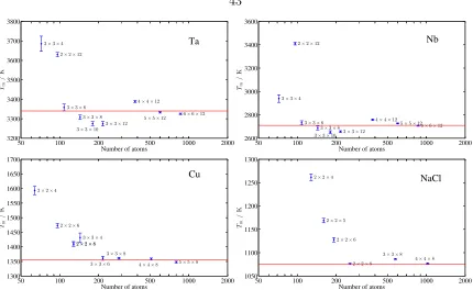
3.3.1 Tantalum at ambient pressure . . . 44
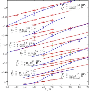
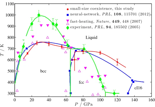
3.3.2 Sodium phase diagram under high pressure . . . 48
3.3.3 NaCl at ambient pressure . . . 51
3.4 Discussions . . . 53
3.4.1 Advantages: robustness, accuracy, speed, etc. . . 53
3.4.2 Disadvantages: finite-size error, slow kinetics, and configura-tional entropy . . . 55
3.4.3 Pulay stress . . . 59
3.5 Code development . . . 60
3.6 Conclusions . . . 60
4 Melting properties of lanthanum zirconate (La2Zr2O7) 62 4.1 Methodology . . . 64
4.1.1 Computation . . . 64
4.1.2 Experiment . . . 65
4.2 Melting and thermal properties . . . 66
4.2.1 Fusion enthalpy . . . 66
4.2.2 Melting temperature . . . 67
4.2.3.1 Oxygen sublattice . . . 71
4.2.3.2 Cation sublattice . . . 74
4.2.4 Heat capacity . . . 77
4.2.5 Thermal expansion . . . 78
4.3 Conclusions . . . 79
5 Design and search of novel refractory materials 80 5.1 Hf-C system . . . 81
5.2 Hf-Ta-C sytem . . . 85
5.3 Hf-C-N system . . . 86
5.4 Conclusions . . . 91
6 Conclusions 92
List of Figures
1.1 Traditional large-size coexistence method . . . 2
1.2 Fast-heating method (Z-method) . . . 3
1.3 Two-phase thermodynamics method . . . 6
2.1 (a) Probability density ρ(∆U) and the product ρ(∆U) exp −∆U/kT of liquid copper at 2000 K; (b) Volumetric display of the insertion energy 13 2.2 Diagrammatic illustration of the algorithm . . . 14
2.3 Nearest neighbor distance analysis of liquid copper at 2000 K . . . 15
2.4 Finite-size correction to the calculation of chemical potential . . . 20
2.5 Determine melting point from chemical potential curves intersection . . 23
2.6 Two-dimensional energy surface illustrating why our four-step algorithm works more efficiently than pre-screening . . . 24
2.7 Finite size error of chemical potential calculations . . . 27
2.8 Convergence tests carried out on different grids . . . 28
2.9 Correlation between insertion energy and size of cavity . . . 29
3.1 Schematic illustration of small-size coexistence method . . . 33
3.2 (a) EnthalpyH versus time tof 50 independent MD systems (6×6×12 supercell, 864 atoms) at 3325 K; (b) The melting properties fitted . . . 33
3.3 Free energy profile and probability distribution of the final states . . . 34
3.4 Transition rate based on transition state theory . . . 34
3.5 lx as a function of cell length l in supercell size 9×9×l . . . 41
3.6 Finite-size effect caused by system size n in n×n×l . . . 42
3.8 Various tests on different materials to study the finite-size effect . . . . 43
3.9 The impact from box size a×a×2a on the error . . . 44
3.10 The melting properties fitted . . . 45
3.11 Comparison of PBE-core, PBE-valence, and PW91-core . . . 46
3.12 N V E MD simulation of solid-liquid coexistence with 864 Ta atoms . . 48
3.13 The melting temperatures of bcc and fcc Na up to 120 GPa . . . 49
3.14 Comparison of our results with other theoretical and experimental studies 50 3.15 Traditional large scale coexistence method (N V E) at differentE . . . 52
3.16 The melting properties of NaCl . . . 52
3.17 Difference between pure-solid and solid-liquid coexistence SQS’s. . . . 58
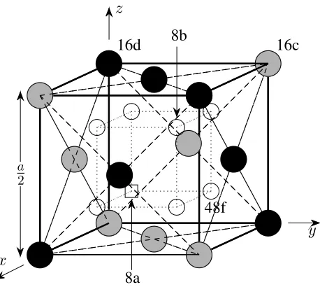
4.1 Pyrochlore structure of La2Zr2O7 . . . 64
4.2 Melting and crystallization of La1.96Zr2.03O7 in thermal analyzer . . . . 66
4.3 The melting temperature of La2Zr2O7 . . . 68
4.4 Potential energy upon perturbation along a soft mode . . . 70
4.5 (a) Distance to ideal pyrochlore position during MD simulation; (b) Potential energy diagram based on nudged elastic band (NEB) method 72 4.6 Synchrotron X-ray diffraction of La2Zr2O7 . . . 76
4.7 Heat capacity of pyrochlore La2Zr2O7 up to melting temperature . . . 77
4.8 Lattice parameter in MD simulation and X-ray diffraction experiment . 78 5.1 Hf-C phase diagram . . . 82
5.2 Wavefunctions illustrating the diversity of bond types in HfC . . . 82
5.3 Electronic density of states in HfC . . . 83
5.4 Electron transfer in HfC . . . 83
5.5 Melting temperature of TaxHf1−xC0.875 as a function of x; inset: the effect on the Fermi level of the solid phase by tuning composition . . . 85
5.6 Melting temperatures of Ta-Hf-C-N alloys . . . 88
5.7 Heat of fusion in Hf-C and Hf-C-N systems . . . 90
List of Tables
2.1 Comparison of differentk-space sampling in terms of computational cost
and error . . . 18
2.2 Calculation of Helmholtz free energy change ∆FN→N+1 . . . 19
2.3 Theoretical chemical potential of liquid copper . . . 21
2.4 Enthalpies and chemical potentials of liquid copper . . . 22
3.1 Melting properties and comparison with benchmarks . . . 39
3.2 Melting properties and comparison with benchmarks . . . 45
3.3 Comparison of PBE-core, PW91-core, and PBE-valence . . . 47
3.4 Melting temperature and volume change at different pressures . . . 49
3.5 Computational costs of our method and traditional coexistence approach 54 4.1 Experimental and calculated structures of La2Zr2O7. . . 65
4.2 HSE correction on melting temperature . . . 68
4.3 Comparison with experimental melting temperature . . . 69
4.4 Pair correlation as an order parameter to quantify the randomness of newly formed solid from MD . . . 74
5.1 HSE correction on melting temperature . . . 81
5.2 Melting temperatures from small-cell coexistence calculations . . . 87
Chapter 1
Introduction
Theoretical predictions of melting temperature have a long history [1], and have
been based on a wide variety of computational approaches, as well as different levels
of accuracy in the descriptions of interatomic interactions. In the last two decades,
thanks to the increased availability of computing power, density functional theory
(DFT) [2, 3, 4] has established itself as a useful simulation tool for accurate and
general modeling of materials. However, melting point predictions based on DFT
are still considered challenging because of the requirement for large simulation cells,
long simulation trajectories, and/or the dependence on auxiliary empirical potentials.
In this chapter, we first review a number of commonly used methods. Through
comparison, we summarize several key favorable features that an ideal method should
contain. These discussions lead us to develop two methods, i.e., the Widom’s
test-particle insertion method and the small-cell coexistence method, which are extensively
studied in this thesis.
1.1
A review of current methods
Over the past decades, numerous ingenious methods have been devised to capture
melting temperatures from DFT. Some of them are inspired by the natural process of
melting: the melting temperature is approached by the evolution of the solid and/or
the liquid involved in the phase transition. The atomic movements are simulated
0 1 2 3 4 5 6 7 8 1330
1340 1350 1360 1370 1380 1390 1400 1410
Time / ps
Temperature / K
Temperature Time average
Figure 1.1: Traditional large-size coexistence method. This figure shows the tem-perature evolution over time. After 3 picoseconds, the system reaches equilibrium, and thus the stabilized temperature is the melting point. Here a Cu embedded atom model (EAM) potential (Mendelev, 2008) [5] is employed on a 40×20×20 face-center cubic (fcc) supercell, with 64,000 atoms.
locate melting temperatures based on thermodynamic properties, e.g., the free
ener-gies of the solid and the liquid. Here we review some of the most commonly used
methods to date.
Large-size coexistence method
In the traditional large-size coexistence method [6, 7, 8, 9, 10], people search
for stabilized solid-liquid coexistence, whose temperature is naturally the melting
point. The simulations are usually carried out in a N V E (or N P H) ensemble, i.e.,
constant number of atomsN, constant volumeV, and constant internal energyE. To
understand how this technique helps the system evolve toward equilibrium, consider a
coexisting system with a phase boundary. If the system as a whole is at a temperature
slightly below the melting point, then some portion of the liquid phase will solidify, generating the appropriate latent heat. Because the system is closed (N V E), this heats up the system towards the melting point. Similarly, if the system is above the melting temperature, the latent heat required to melt the solid will cool the system
down. There is no difficulty in nucleating either the liquid or solid phases, as the
interface assists the nucleation for the melting or solidification process. In the N V E
0.8 1 1.2 1.4 1.6 1.8 2 2.2 2.4 2.6 500
1000 1500 2000 2500 3000
Pressure / kbar
Temperature / K
melting
solid
liquid
energy increase
Figure 1.2: Fast-heating method (Z-method). This figure shows the temperature-pressure relation during the heating process. A Cu EAM potential (Mendelev, 2008) [5] is employed with 32 atoms in the system. Here N V E ensembles are simulated at different values of E. The melting temperature is located in the region where the temperature drops abnormally as more energy is put in. This figure also presents another problem of the method: Z-method melting occurs in a wide temperature range and hence the melting temperature is indefinite.
and liquid can coexist; the average temperature and pressure along the simulation
then provide a point on the melting curve. If the energy E is above/below the range
where coexistence can be maintained, the system will completely melt/solidify, and
the simulation does not provide useful melting properties information.
The large-size coexistence is an accurate method, provided that the system size is
sufficiently large. However, DFT calculations on such large systems are prohibitively
expensive. To stabilize solid-liquid coexistence, it typically requires a cell with at least
1,000 atoms. Moreover, it usually takes at least thousands of MD steps to equilibrate
the coexistence, which renders the cost skyrocket.
Fast-heating method (Z-method)
The fast heating method [11, 12, 13, 14] attempts to resemble how melting points
are measured in common experiments. The procedure starts with a small cell of the
solid at a low temperature. Then the temperature is gradually increased, with the
crystal melts. It is straightforward to determine the melting temperature because the
latent heat during melting causes a temperature drop.
While the method is both simple and fast, it suffers from serious drawbacks [13,
15, 16]. Real melting in nature is usually initiated at surfaces and crystal defects. By
comparison, melting in a defect-free periodic bulk solid is by no means the same. This
so-called “homogeneous melting” has a widely acknowledged feature: superheating
and hysteresis. The solid will remain in a metastable solid phase until the temperature
is far above the true melting point. The reason for superheating is apparent. In order
to initiate the nucleation of a liquid, the defect-free crystal needs extra energy (or
temperature, correspondingly) to form a defect, the nucleation center. The amount
of extra energy determines the extent of superheating, and hence the calculation
error. Another related problem is about timescales, i.e., the kinetics of homogeneous
melting. The chance to form a nucleation center depends not only on the activation
energy, but also the amount of time elapsed. This relation leads to an annoying
requirement of the method: very long MD trajectories are needed and they are never
guaranteed long enough.
Free energy method
The free energy method [17, 18, 19, 20, 21] relies on separate calculations of the
free energies of the solid and the liquid, and determines the melting temperature by
locating the intersection of the two free energy curves. Among them, the liquid-state
free energy calculation is the most difficult component [22]. Here we describe two
typical methods.
• Thermodynamic integration method
This method first calculates the free energy based on empirical potentials (e.g.,
by Widom’s test-particle insertion method). Then in order to bridge the gap
between the empirical potentials and DFT, a general technique called
“thermo-dynamic integration” is carried out to determine the free energy correction. The
by isothermally switching the atomic interactions from the empirical potentials
(Hα) to DFT (Hβ).
µβ =µα+ 1
N Z 1
0
Hβ −Hα
λdλ. (1.1)
Here α and β are the empirical potentials and DFT, respectively. µ is free
energy (chemical potential), and N is the number of particles. h· · · iλ denotes the ensemble average of the Hamiltonian Hλ = (1−λ)Hα+λHβ.
The success or failure of the scheme depends heavily on the quality of the
em-pirical potentials, because it determines the effort needed to compute the free
energy correction µβ −µα [23]. A bad empirical potential would render the thermodynamic integration expensive. This problem becomes even worse in a
complex multi-component system, when a huge number of high-quality
poten-tials are required (e.g., at leastC2
N pairwise empirical potentials for aN-element
system). This requirement limits the application of the method. Furthermore,
the thermodynamic integration method is inherently complicated and difficult
to automate, since it requires a considerable amount of user-computer
interac-tions.
• Two-phase thermodynamics method
This method [24, 25, 26] proposes a two-phase model, which decomposes the
liquid-state phonon density of states (DoS) into a gas phase component and a
solid phase. The gas component mostly contributes in the low frequency regime
and contains all the fluidic effects, whereas the solid component, located at
higher frequencies, has no fluidicity but can possess strong quantum effects. The
liquid-state phonon DoS is easy to compute, and the free energy of a solid/gas
phase is well studied. The choice of the gas phase model is flexible, e.g., hard
spheres. However, a drawback of this method is its low accuracy, especially at
0 5 10 15 x 1012 −1
0 1 2 3 4 5 6 7x 10
−11
ν/ s−1
density of states / s
total gas−like part solid−like part
Figure 1.3: Two-phase thermodynamics method. This figure shows the partitioning of the liquid-state phonon density of states (blue, copper at 2000 K, PBE) into solid-like (red) and gas-like (green) parts whose free energies are straightforward to compute.
fictitious solid and gas components, which is an assumption not always valid.
The liquid is not a combination of a solid and a gas in reality. In addition, the
harmonic approximation employed in free energy calculations becomes poor at
high temperatures, as anharmonic effects start to dominate.
1.2
Our goals
Although these popular methods are successful in a wide range of applications,
they are far from perfect. Our primary goal is to devise methods that deliver a
melting point estimate simply, quickly, and accurately. We summarize as follows a
list of favorable features.
• direct DFT
DFT has clear advantages over its competitors. It is robust and reliable in a very
general range of systems (though under some circumstances its performance is
limited). It is well balanced between accuracy and computational cost,
provid-ing relatively high accuracy with a modest computer demand. We believe an
thermodynamic integration method. A direct DFT method is also simpler and
easier to implement and automate.
• highly automated
A highly automated approach reduces human effort and makes possible
multi-tasking, i.e., to calculate melting points on several materials concurrently. With
the increasing availability of computer power, this feature becomes more and
more attractive when a task involves a large number of melting point
calcula-tions, such as solid-liquid phase diagram calculations and material screenings.
Direct DFT is a key element to achieve automation: it takes considerable
hu-man effort to develop or search for empirical potentials. The difficulty varies
to automate a method. For example, while the fast-heating method is
straight-forward to implement and automate, the thermodynamic integration method is
inherently complicated and it requires heavy human input.
• fast and accurate
These are essential features.
• robust and flexible
A robust method is likely to remain effective when the environment changes.
For example, the direct connection to DFT suggests general robustness in terms
of atomic interactions. Another favorable feature is the ability to achieve high
accuracy in several stages: low accuracy can be achieved at a low cost, and the
accuracy can be improved systematically when more calculations are performed.
This flexibility is ideal for material screening efforts.
In the next two chapters, we introduce two new methods: (1) an improved version
of the Widom’s particle insertion method based on high selectivity in carrying out
DFT calculations on insertion energy, and (2) the small-cell coexistence method,
which captures melting temperature from statistical analysis of duplicated
small-cell solid-liquid coexistence simulations. Both methods operate through direct DFT
and accurate. In particular, the small-cell coexistence approach is robust and easy to
Chapter 2
Widom’s particle insertion
Widom’s test-particle insertion scheme [27] is a popular method to directly calcu-late the chemical potential of a liquid. Chemical potential is calcucalcu-lated as additional
free energy, specifically, a change of free energy after inserting one more particle.
Consequently, the chemical potential is related to the ensemble average and
integra-tion of Boltzmann’s factors exp (−β∆U), where ∆U is insertion energy, the energy change during particle insertion. In practice, the average is evaluated by occasionally
inserting the test particle into the simulation volume, measuring ∆U, and then
re-moving it before continuing the simulation. This approach has been applied to some
simple empirical potentials [28, 29, 30, 31, 32], mostly Lennard-Jones potentials. The
major problem of the Widom method is that it is usually considered computationally
too expensive, because most insertion attempts lead to a vanishingly small value of
exp (−β∆U) (due to the high energy cost of inserting the test-particle in a small cavity in the dense system) and the corresponding computational efforts are thus
wasted. Probably because of the prohibitive computational cost, there have
appar-ently been no attempts so far to compute first-principles chemical potential directly
with Widom’s method.
Nevertheless, compared to the thermodynamic integration approach, the Widom
method holds a great advantage, since it does not require any reference system. This
property makes it possible to find a universal solution to first-principles calculations of
liquid-state chemical potentials. This is especially useful in the automated materials
need to develop empirical potentials for each of the chemical system explored. In this
chapter, we revisit Widom’s particle insertion method and modify it with an efficient
cavity-sampling scheme, which achieves a drastic reduction in computational cost.
2.1
Methodology
2.1.1
Particle insertion method
We briefly reiterate the Widom particle insertion method here. By definition,
chemical potential µis the partial derivative of free energy F with respect to number
of particles N, µi =
∂F ∂Ni
V,T ,Nj6=i
, where V is volume and T is temperature. Thus
it can be calculated by evaluating the additional free energy, namely the free energy
change after inserting one more particle.
µi =F(V, T, Ni+ 1, Nj6=i)−F(V, T, Ni, Nj6=i) +O
∂2F
∂N2
i
!
. (2.1)
The higher-order derivative, which leads to finite-size correction, will be discussed
later in Section 2.2.1. Assume the system of interest containsN homogeneous atoms.
The Helmholtz free energy of such a system is (using a classical partition function)
F(V, T, N) =−kT ln
1 Λ3NN!
Z
exp
"
−U(r
N)
kT #
drN
, (2.2)
where k is the Boltzmann constant, Λ is de Broglie wavelength, Λ =ph2/(2πmkT),
andU is potential energy. Combining Eq. (2.1) and (2.2), the expression for chemical
potential can be written as
µ ' ∆FN→N+1 =µid+µex, (2.3)
µid = −kTln
V
Λ3(N + 1)
, (2.4)
µex = −kTln 1
V R
exp
−U(rN+1)/kT
drN+1
R
exp−U(rN)/kT
drN
!
Notice that the approximation sign in Eq. (2.3) is due to the omission of the
higher-order derivative in Eq. (2.1), which we will discuss and correct later.
In Eq. (2.3), we separate the chemical potential into two parts, the ideal gas term
µidand the excess termµex. The chemical potential of ideal gas is trivial to calculate.
To compute the excess part µex, we further write it as an ensemble average:
µex =−kTln
1 V * Z exp
−∆U
kT
drN+1
+
N
, (2.6)
where ∆U is the potential energy change during insertion, ∆U(rN,rN+1) =U(rN+1 = {rN,r
N+1})−U(rN). Notice the difference betweenri andrN. ri denotes the position
of theith atom, while rN contains the coordinates of all atoms in the configuration, which has a dimension of 3N. The notation h· · · iN means the canonical ensemble average of a N-particle system
hAiN =
Z
Aexp−U(rN)/kT
drN
Z
exp−U(rN)/kT
drN
. (2.7)
In practice, the evaluation of Eq. (2.6) involves the calculation of two averages,
namely the ensemble averageh· · · iN and the spatial average 1
V Z
exp −∆U/kTdrN+1. The ensemble average can be achieved by picking snapshots of configurationsrN
ran-domly from MD or MC trajectories, while the spatial average is calculated by
thor-oughly scanning over rN+1, the position of the additional particle, in each snapshot.
2.1.2
Selective sampling
An obvious way to calculate the spatial average would be to carry out a uniform
random sampling of the additional particle in the rN+1 space. However, this is not a very practical approach. In practice, one can sample only a limited number of
positions, and few of them would actually fall in the low energy region of interest.
wasteful. Therefore an efficient sampling scheme is essential to avoid the
random-sampling catastrophe.
It is more useful to regard the average in Eq. (2.6) as a one-dimensional integral
over the insertion energy ∆U, i.e.,
µex =−kT ln
Z +∞
−∞
ρ(∆U) exp
−∆kTU
d(∆U)
!
, (2.8)
where ρ(∆U) is the probability density defined as
1
V Z
δ(U({rN,rN+1})−U(rN)−∆U) drN+1
N
. (2.9)
Notice again that h· · · iN is the canonical ensemble average of a N-particle system, according to Eq. (2.7).
In order to determine accurately the right-hand side of Eq. (2.8), one has to
produce good estimates of the values of ρ(∆U) for the range of ∆U over which the
productρ(∆U) exp −∆U/kTtakes on its large values. In other words, the sampling should be exclusively focused on the region near the cavities that can accommodate
the additional particle at a small energy cost.
Here we give an example of liquid copper at 2000 K. (see Fig. 2.1) Since chemical
potential is determined by the area below the curve ρ(∆U) exp −∆U/kT, which decays exponentially in high-∆U region, we introduce here an energy ceiling (e.g.,
∆U = 0.6 eV in the figure) to focus on the study of low-∆U region, ignoring
the rest. The energy ceiling is simply determined as a value where the product
ρ(∆U) exp −∆U/kTbecomes negligible, thus the converged excess chemical poten-tialµex is captured at the lowest computational cost, which is proportional to the area
below the probability density curve. (Throughout the text, we choose as reference
state (zero level in energy) the enthalpy of Cu(s) at 298 K and zero pressure, which
−1.5 −1 −0.50 0 0.5 1 1.5 2 1
2 3 4x 10
−3
energy ceiling
S1
S2
µex=−kT lnS1
cpu cost∝S2
ρ e − ∆ U / k T / eV − 1
∆U / eV ρe−∆U/kT
ρ
−1 0 1 20
0.4 0.8 1.2 1.6 x 10⁻³
ρ / eV − 1 (a) 1.5 1 0.5 0
∆U / eV −0.5
−1 −1.5
(b)
Figure 2.1: (a) Probability density ρ(∆U) and the product ρ(∆U) exp −∆U/kT
of liquid copper at 2000 K. (b) Volumetric display of the insertion energy ∆U for a single snapshot in configuration rN. The colored region with low ∆U contribute
most to the chemical potential, despite of its small size and correspondingly modest computational cost, compared to the whole cube.
2.1.3
Algorithm
We propose here an algorithm to efficiently find the cavities and calculate the
spatial average. For a N-particle configuration rN0 in a parallelepiped, the integral can, in principle, be evaluated numerically on a uniform grid:
1
V Z
exp −∆U(r
N
0 ,rN+1)
kT
!
drN+1 (2.10)
= 1
NaNbNc Na,b,c
X
i,j,k=1
exp −∆U(r
N
0 ,rN+1 =rijk)
kT
!
,
where
rijk =
i Na
a+ j
Nb
b+ k
Nc
c. (2.11)
a, b, c are the vectors defining the parallelepiped. Instead of running ab initio calculations on all grid points, we employ the following algorithm to search for cavities
and to study the potential energy surfaces near them.
r
0 r1 r2
r 3 r4
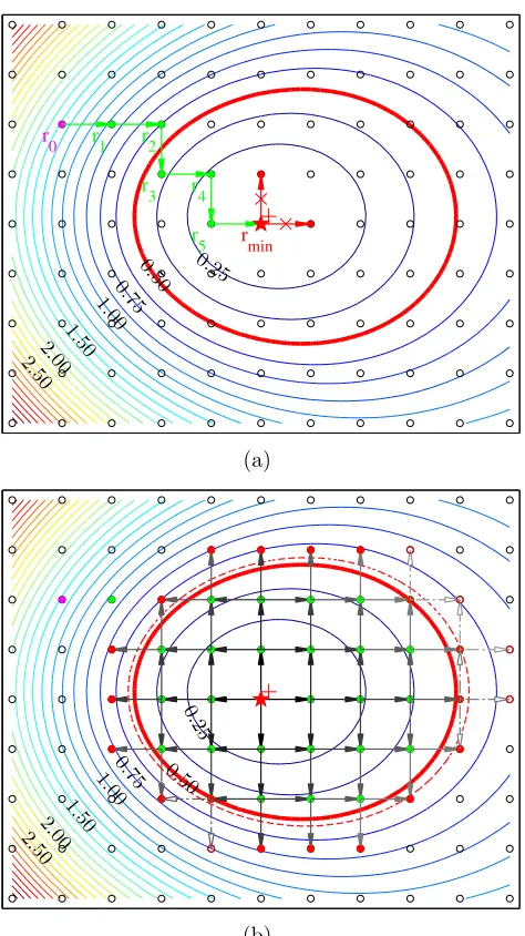
[image:27.612.206.443.72.494.2]r 5 rmin 0. 25 0. 50 0. 75 1. 00 1. 50 2. 00 2. 50 (a) 0. 25 0. 50 0. 75 1. 00 1. 50 2. 00 2. 50 (b)
Figure 2.2: Diagrammatic illustration of the algorithm in two dimensions. Assume the contour lines above represent the energy surface near the cavity we are interested in. (a) Step 1: We first estimate the position of the cavity (purple, rN+1,0) based on an approximate energy function. Step 2: Then DFT calculations are carried out and, based on the force calculated, the position of the (N+ 1)th particle (green,rN+1,i) is
optimized until the minimum grid point (red star, rN+1,min) is found. The optimiza-tion proceeds as move attempts are accepted if U({rN0 ,rN+1,i+1})< U({rN0 ,rN+1,i}).
The green arrows are accepted move attempts, while the red ones are denied. (b) Step 3: All grid points below the energy ceiling (red circle) are studied with DFT, by gradually climbing up the energy surface from the bottom, until all frontier points (red solid dots) are above the energy ceiling. As a result, we need to calculate ∆U
−1.5 −1 −0.5 0 0.5 1 1.5 1.8
2 2.2 2.4 2.6
∆U / eV rm
in
/
˚ A
Figure 2.3: Nearest neighbor distance analysis on 256 configurations rN of liquid
copper at 2000 K. The nearest neighbor distance rmin is calculated as the shortest distance from the grid point rijk to the N atoms and their periodic images. Large
rmin corresponds to the center of a large cavity, which is optimal for particle insertion at a low energy cost.
find this cavity and map out the nearby potential energy surface in four steps.
1. Locate: We first estimate the position rN+1,0 of the cavity based on an approx-imate energy function. This function should tell us roughly where the cavity
is, but does not need to be accurate, because it is never used to calculate the
chemical potential. There are plenty of choices available to take this task. For
example, an appropriate empirical potential is definitely sufficient to predict the
position of the cavity. In practice, we find that even a function as simple as
nearest neighbor distance can help locate the cavity, as shown in Fig. 2.3. This
idea of prescreening has been successfully used before [33, 34].
2. Minimize: DFT calculation is performed at the predicted positionrN+1,0. Based on the force calculated on the (N + 1)th particle, the position is optimized
as rN+1,1. This move attempt is checked by DFT, and will be accepted if
U({rN0 ,rN+1,1}) < U({rN0 ,rN+1,0}). The optimization continues and generates
a series of positions {rN+1,i, i = 1,2,· · · } until the minimum is found. This
procedure is equivalent to structure optimization under the constraint that all
atoms are fixed except the last one, which is allowed to move only on grid points.
surface. If the bottom is lower than the energy ceiling, all its neighboring grid
points will be studied. And if some of them are also below the ceiling, their
neighbors will also be further calculated. This procedure spreads the “seeds”
out, until all “seeds” hit the energy ceiling, which tells us that we have reached
the inaccessible space region and there is no need to explore any more. The
exploration will end only if all points on the frontier of the cavity are above the
energy ceiling.
4. Converge: An appropriate value for the energy ceiling is required in Step 3.
However, unlike what has been discussed in Fig. 2.1, the probability density
ρ(∆U) is never known before we calculate it, rendering the energy ceiling a priori unknown. We circumvent this problem by introducing a dynamic, rather than static, energy ceiling. Starting from a relatively low trial value (e.g., −0.5 eV in Fig. 2.1), we first calculate the probability density below it (by Step 3),
and then decide whether or not we should raise the energy ceiling, depending on
the up-to-date ρ(∆U) exp −∆U/kT. The new energy ceiling, if it happens, may enclose some of the frontier points, thus restarting the exploration of the
cavity (returning to Step 3). After the additional calculation is finished, the
same question is asked again about whether to further increase the energy
ceil-ing. Step 3 and Step 4 are performed repeatedly, increasing the energy ceiling
gradually and mapping out Fig. 2.1 from left to right, until the energy
ceil-ing is high enough to give an excess chemical potential converged within some
2.2
An application: chemical potential and
melt-ing temperature of copper
2.2.1
Chemical potential of liquid copper at 2000 K
We employ the scheme described above to calculate the chemical potential of liquid
copper from first-principles. Before we describe the detailed methodology, we would
like to first estimate the precision required in our calculation, because we want to
further apply the results to theoretical prediction of material properties, e.g., locating
a melting point. We notice that the calculation of melting properties demands very
high precision for chemical potentials. The melting temperature is determined by the
intersection of chemical potential curves of a solid and a liquid. However, in practice
these two curves usually cross at a shallow angle. Consequently, a small error in
chemical potential may translate into a relatively large error in melting temperature.
Typically, an error of 10 meV in chemical potential will result in an error of 100 K in
melting point. Therefore, we need to make sure numerical and statistical errors are
under control.
In the process of isochoric particle insertion, we use a periodic cube of edge length
11.66 ˚A with 108 copper atoms in it. All DFT calculations are performed using the
VASP package [35, 36], with the projector-augmented-wave (PAW) implementation
[37, 38] and the generalized gradient approximation (GGA) for exchange-correlation
energy, in the form known as Perdew-Burke-Ernzerhof (PBE) [39]. Electronic
tem-perature and its contribution to entropy are counted by imposing Fermi distribution
of the electrons on the energy level density of states. The size of the plane-wave basis
is carefully checked to reach the required accuracy. The energy cutoff (Ecutoff) is set
to 273 eV in MD runs and particle insertion attempts. When we make corrections
for pressure and energy,Ecutoff is increased to 500 eV in order to remove Pulay stress
(error in pressure within 1 kbar) and achieve convergence (error in energy within 1
meV) with respect to the basis size.
ac-Table 2.1: Comparison of different k-space sampling in terms of computational cost and error (in unit of meV/atom).
k-space sampling number error in MD error in ∆U
Γ point 1 46 106
MP 2×2×2 4 2 6
MP 4×4×4 32 <0.1 1
8 special k-pointsa 8 <0.1 3
4 special k-pointsb 4 0.5 19
a. The coordinates of the k-points are:
(1/8 1/8 1/8), (-3/8 1/8 1/8), (1/8 -3/8 1/8), (-1/8 -1/8 3/8), (-1/8 3/8 3/8), (3/8 -1/8 3/8), (-3/8 -3/8 1/8), (3/8 3/8 3/8). b. The coordinates and weights of the k-points are:
(1/8 1/8 1/8), 1/8; (3/8 1/8 1/8), 3/8; (3/8 3/8 1/8), 3/8; (3/8 3/8 3/8), 1/8
curacy and computation cost. A densek-point gird is necessary to meet the accuracy
requirement. Indeed, we would like to use a 4×4×4 Monkhorst-Pack(MP) mesh in the first Brillouin zone (FBZ). However, since the point-group symmetry of our
cubic supercell is broken by disorder, this would require all the 32 k-points included
in the calculation, which is computationally too demanding. Kresse et al. [18] have addressed this problem by replacing the original 32k-points with four specialk-points
in the irreducible FBZ, as if full cubic symmetry were still applied. This reduction
can be well justified by the following argument. In the case of weak potential and
nearly free electron gas, the dominant part in electronic Hamiltonian is the kinetic
energy, which is approximately ¯h2/(2me)(G+k)2 (G is a reciprocal lattice vector
and k a k-point in FBZ), a term invarient under point-group operation with respect
to the choice of k. As simple metals are close to the free electron gas model, the
same property should hold true, thus rationalizing the reduction of k-points by
sym-metry. Inspired by this idea and making a further improvement in which we seek
a relatively even distribution of k-points in FBZ (while in Kresse et al.’s calcula-tion, the k-space sampling focuses exclusively in the first octant), we represent the
4×4×4 MP grid by eight special k-points, whose coordinates are listed in Table 2.1. To evaluate the accuracy, different k-space sampling methods are tested on ten
Table 2.2: Calculation of Helmholtz free energy change ∆FN→N+1 by particle inser-tion.(Cu, 2000 K,N = 108, a= 11.66˚A, in eV)
µex 0.748±0.011
µid −2.021
∆FN→N+1 −1.273±0.011
(calculated as ∆U =U(rN+1)−U(rN)). As Table 2.1 shows, sampling with the eight specialk-points is comparable to the 4×4×4 MP grid, while the computational cost is significantly reduced by a factor of four.
The ensemble average is computed numerically by running ab initio MD simu-lations within a canonical (NVT) ensemble with the Nos´e-Hoover chain thermostat
[40, 41, 42, 43]. The MD simulation proceeds with a time step of 3 femtoseconds and
lasts for 1280 steps. Forces acting on atoms are accurately calculated, as the
conver-gency threshold for electronic structure optimization is set to 1×10⁻⁸ eV/atom. We capture snapshots every 5 ionic steps from the MD trajectory, thus generating 256
snapshots in total, from which the ensemble average is evaluated. The configuration
rN in each snapshot is then studied by making particle insertion attempts in order to compute the spatial average overrN+1. The spatial average is calculated numerically on a uniform 40×40×40 grid, according to Eq. (10). Only on selected grid points are ab initio insertion energies ∆U calculated, following the efficient scheme we pro-posed in Section 2.1.3. Finally, we compute the chemical potential by combining the
ensemble and spatial averages.
As shown in Table 2.2, we “measured” the chemical potential of liquid copper at
2000K five times, based on five independent MD trajectories. The Helmholtz free
energy change during particle insertion ∆FN→N+1 is−1.273±0.011 eV.
The selective calculation scheme helps us reduce the computational cost
drasti-cally. Instead of runningab initio calculations on all 1.6×10⁷ grid points, the scheme demands calculations on only 5×10³ grid points, reducing the computational cost by a factor of 3×10³ and thus making the computation possible.
Now we make correction for the finite-size effect, which was alluded to earlier in
N, T, p1, V particle insertion isochoric
µ(V, T, N) = ∆FN→N+1−(p2−p1)·V /(2N) N+ 1, T, p2, V
Figure 2.4: Finite-size correction to the calculation of chemical potential by isochoric particle insertion method.
this type of correction. Despite the differences, they all share the same leading term,
− 1 2N ∂p ∂ρ
, where ρ is the density of particles. Here we would like to account for
the finite-size effect in the following way. The flaw of isochoric particle insertion lies
in the fact that the next higher-order derivative may be significant and has to be
included, which can be seen from the following Taylor expansion:
∆FN→N+1 = F(V, T, N + 1)−F(V, T, N)
.
= µ(V, T, N) + 1 2
∂µ(V, T, n)
∂n
n=N
, (2.12)
where ∆FN→N+1is the free energy change computed from particle insertion,µ(V, T, N) is the exact chemical potential, and (∂µ/∂n) is the leading correction term. Notice
that this term is large for condensed phase materials, i.e., when n increases, µ will
change significantly, as a result of the large increase in pressure. Simplifying the
expression, we have the finite-size correction
∂µ(V, T, n)
∂n =
∂µ(p, T)
∂p ·
∂p(V, T, n)
∂n =
V
N(p2 −p1), (2.13)
µ(V, T, N) = ∆FN→N+1−
V
2N(p2−p1), (2.14)
where p1 and p2 are the pressure before and after particle insertion, as shown in Fig.
2.4.
It is straightforward to show that this correction is equivalent to− 1 2N ∂p ∂ρ , the
leading term in the corrections proposed by Smit [44] and Siepmann [45].
−2VN(p2−p1) = −
V
2N
∂p(V, T, n)
∂n =−
1 2N
∂p(V, T, n)
Table 2.3: Theoretical chemical potential of liquid copper at 2000 K.(in eV, N = 108, a= 11.66˚A, p1 = 5.5 kbar, p2 = 10.6 kbar)
∆FN→N+1 −1.273±0.011 −(p2−p1)V /(2N) −0.023
−p1V /N −0.050
µ(p◦,2000K) −1.347±0.011
µ(p◦,2000K,exp.) −1.342
Another type of finite-size effect can be understood as the following. Compared
to an infinite system, the test particle inserted in a small box will interact with its
periodic images. In the case of charged atoms, the image charge interaction can be
very large due to the long-range Coulomb interaction. In our small periodic model,
image interactions must be examined to make sure that they are small enough to be
neglected. To estimate this effect, we perform particle insertion tests on a 864-atom
system (eight times larger than our original model) and make comparisons with the
original results. The calculated insertion energies ∆U differ only by less than 3 meV.
Thus it is safe to neglect the weak image interactions in our model.
We have now calculated µ(p1,2000K). We further convert µ(p1, T) to µ(p◦ = 1 bar'0 kbar, T), the chemical potential at standard atmospheric pressure, to sim-plify the comparison of our theoretical results with experiments.
µp1→p◦ =µ(p
◦, T)
−µ(p1, T)' −
p1V
N . (2.16)
The chemical potential is finally computed by combining Widom’s particle
inser-tion method and the correcinser-tions for finite-size effect and non-zero pressure.
µ(p◦, T) = ∆FN→N+1−
V
2N(p2−p1)− p1V
N . (2.17)
Table 2.4: Enthalpies and chemical potentials of liquid copper. (in eV/atom)
T H Hexp µ µexp
2000 - - −1.347±0.011 -1.342
1950 0.642 0.645 −1.297±0.011 -1.292 1850 0.609 0.611 −1.198±0.010 -1.194 1750 0.575 0.577 −1.102±0.010 -1.097 1650 0.540 0.543 −1.007±0.009 -1.002 1550 0.505 0.509 −0.914±0.009 -0.910 1450 0.470 0.475 −0.824±0.008 -0.819 1350 0.434 0.441 −0.736±0.008 -0.731
2.2.2
Chemical potential at various temperatures
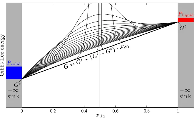
The Gibbs free energies G at different temperatures and pressures are connected
by the following thermodynamic relations:
∂(G/T)
∂(1/T)
p
=H,
∂G
∂p
T
=V. (2.18)
Since enthalpy H and volume V can be obtained directly from MD simulation, free
energy changes among different (p, T) conditions can be readily computed by the
thermodynamic integration method.
We start from the calculated µ(p◦,2000 K) and map out the chemical potential curve in regionT ∈[1300,2000] K and zero pressure. To compute enthalpyH in Eq. (2.18), ab initio canonical (N V T) MD simulation is performed at various tempera-tures in the region. Detailed settings in DFT calculations and MD thermostat have
been described in Section 2.2.1. Enthalpy is calculated as the average of energies over
MD trajectory at each temperature. Volume search is conducted to make surep'0 kbar. As shown in Table 2.4, the calculated enthalpy and chemical potential agree
very well with experiments.
2.2.3
Calculation of melting temperature
The chemical potential of liquid copper is further used to calculate the theoretical
1300 1350 1400 1450 1500 −0.84
−0.82 −0.8 −0.78 −0.76 −0.74 −0.72
−0.7 µsolid,theory
µliquid,theory
µsolid,exp
µliquid,exp
T / K
µ
/
eV
1360 K (µs,exp=µl,exp)
1440 K (µs,theory=µl,theory)
Figure 2.5: Determine melting temperature from where solid and liquid chemical potential curves intersect on a µ-T plot. Tm from experiments is 1360 K. According to the liquid chemical potential we calculated by Widom’s method, the theoreticalTm is 1320 or 1460 K, depending on whether we use experimental or theoretical results for the chemical potential of solid.
curves of the solid and of the liquid. The chemical potential of solid is computed
within the quasiharmonic approximation [46] and is further corrected by
thermo-dynamic integration (to account for anharmonicity at high temperatures). Phonon
density of states, vibrational free energies, and thermal expansion are calculated
us-ing the “supercell” method as implemented in the Alloy Theoretic Automated Toolkit
(ATAT). [47, 48] Anharmonicity effect is included as further correction through the
thermodynamic integration method, in which MD simulation is carried out with an
effective Hamiltonian
Hλ = (1−λ)Hα+λHβ (2.19)
that gradually switches from the Hamiltonian Hα of a harmonic potential surface to
the real Hamiltonian Hβ. The chemical potential difference is calculated as
µβ =µα+ 1
N Z 1
0
Hβ −Hα
λdλ, (2.20)
where hAiλ is the average of observable A in MD simulation with Hamiltonian Hλ.
The chemical potentials of solid and liquid copper, from both theory and
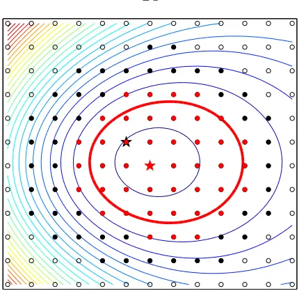
Figure 2.6: This two-dimensional energy surface illustrates why our four-step al-gorithm works more efficiently than pre-screening. While traditional pre-screening labels all colored (both red and black) points as “important” based on the approxi-mate energy model, the “locate” step in our algorithm outputs only the approxiapproxi-mate minimum (a single grid point at the black star). Then the cavity is studied by the “minimize” and “explore” steps relying on ab initio calculations. As a result, our scheme calculates only the red points, and significantly cuts the unnecessary cost (all the surrounding black points).
solid are -5 and -11 meV, respectively, in the melting region. The calculated melting
temperature is 1440 K, about 80 K higher than the experimental value. This error is
translated from both solid and liquid chemical potentials, as a combined effect. Since
we focus mostly on the calculation of liquid chemical potentials in this article, we are
more concerned about the impact purely from the liquid part, which is more accurate
than the solid part and thus should lead to a smaller error. Indeed, the errors in
melting point caused by solid and by liquid are 120 and -40 K, respectively, as shown
2.3
Discussions
2.3.1
Difference with pre-screening
Although the “locate” step in our algorithm appears to be similar to pre-screening,
it is different in many aspects. Working inab initio context, which is computationally much more expensive than empirical potentials, we need to design an algorithm highly
selective about what should be calculated by DFT. In traditional pre-screening, the
approximate energy model is used to find an approximate cavity that must completely
enclose the true cavity, so the pre-screening criterion must necessarily be
conserva-tive and the more accurate/expensive energy model is invoked too often. The key
distinction in our scheme is that the approximate energy model is only used to find
a trial point at or near a cavity. The shape of the cavity is instead determined in the
“explore” step, relying on ab initio calculations, and the only “wasted” calculations are those immediately at the boundary of the cavity. In traditional pre-screening
the set of “wasted” calculation points is three-dimensional, while in our scheme it is
two-dimensional. An example is shown in Fig. 2.6. We save costs on several layers
of black points that are labeled as “important” by pre-screening but proven to be
unnecessary by our algorithm.
One may argue that near the boundary of the cavity there could exist multiple
minima, which could be ignored by mistake in our algorithm. Although it is true
theoretically, this is very unlikely to happen in reality. First of all, if the multiple
minima are connected by a path lying below the energy ceiling, we will not miss them
in the “explore” step. In the case of multiple minima not connecting, we will miss
them only if the “locate” step provides a single starting point when there should
have been more than two. This is not only very rare but also insignificant, because
only small-size shallow cavities can escape from the examination of the “locate” step.
Furthermore, the multiple minima issue is more a numerical convergence aspect than a
fundamental limitation. As the ceiling is dynamically increased up to convergence, all
minima that were previously missed will eventually be connected to existing cavities
2.3.2
DFT error
Although the absolute error in DFT energies is likely larger than our target
accu-racy of 10 meV/atom, we benefit from the fact that our results (the melting point and
chemical potentials relative to a reference state) are actually functions of energy
dif-ferences between states of similar atomic densities and average coordination number,
so that considerable error cancellation is to be expected.
Potential DFT errors aside, we are very careful about controlling the errors both
from numerical and statistical origins. The errors in the ab initio calculations are mainly due to electronic structure calculations implementation details, e.g., the use
of PAW method, the size of basis set and k-space sampling. These problems have
been carefully handled and discussed either in the above paragraph or in Section
2.2.1. The errors in statistical methods are caused by detailed physical approaches to
calculate the chemical potentials of the solid and of the liquid, i.e., quasi-harmonic
approximation, thermodynamic integration, and Widom’s particle insertion method.
Because the chemical potentials of the two phases are calculated with different
statis-tical mechanics methods, we have to make sure that the calculations achieve absolute
convergence with respect to the methods, since there is no chance that errors of the
two phases will cancel.
2.3.3
Finite-size error
Due to computational cost issues of DFT calculations, our chemical potential
cal-culations can be performed only on a small system with around 100 atoms. The error
caused by the small system size is studied systematically, as we gradually increase
the system size and check the convergence. We first note that this error is inherent
in the physical method of particle insertion itself and is irrelevant to the DFT
for-malism. Therefore, it is better to work with empirical potentials, as it is a practical
way to test our method on large system size without losing the accurate description
of interatomic interactions. We implement the particle insertion method into the
0 500 1000 1500 2000 −4
−2 0 2 4 6 8 10 12 14 16 18
Number of atoms
er
ro
r
o
f
µ
/
m
eV
Cu, Mendelev, 2008
Ta, Y. H. Li, 2003
Figure 2.7: Finite size error of chemical potential calculations, tested on two empirical potentials. The errors are 17 and 11 meV for Cu (108 atoms) and Ta (128 atoms), respectively.
to automate and accelerate the calculations. Two embedded atom model (EAM)
potentials, namely copper (Mendelev, 2008) [5] and tantalum (Y.-H. Li, 2003) [50],
are tested on system size up to 2,000 atoms. The results are shown in Fig. 2.7. We
find the chemical potential finally converges after we increase the system size beyond
1,000 atoms. With system size of approximately 100 atoms, the finite size error is
10-20 meV. Considering the huge computation cost we have to pay to work on larger
systems from first principles, this amount of error is still acceptable.
2.3.4
Dependence on numerical grid
The convergence with respect to grid resolution is studied with the same empirical
potentials. We have tested different grid resolutions up to eight times denser than
the grid in our reported DFT calculations. We analyze the results in two levels,
namely the integral I (or spatial average mentioned before in Eq. (10)) in each
individual snapshot and the chemical potential µ according to Eq. (6), which is
related to the ensemble average of the above-mentioned integralsI,µ=−kTlnhIiN. Errors of spatial average in individual snapshots are plotted in Fig. 2.8 (blue cross).
Although for a single snapshot it requires a very fine grid to achieve convergence, the
error mostly cancels out in the ensemble average, therefore the chemical potential
10 20 30 40 50 60 70−2.5 −2 −1.5 −1 −0.5 0 0.5 1 1.5 2 2.5
Ta, Y. H. Li, 2003 chemical potential spatial average
10 20 30 40 50 60 70
−5 −4 −3 −2 −1 0 1 2 3 4 5
10 20 30 40 50 60 70−1
−0.5 0 0.5 1
Cu, Mendelev, 2008
grid resolutionn×n×n
10 20 30 40 50 60 70
−2 −1 0 1 2 er ro r o f µ / m eV ln (
In×
n
×
n
/
I80
[image:41.612.194.450.73.322.2]× 8 0 × 8 0 )
Figure 2.8: Convergence tests carried out on different grids. Results from the densest grid (80 ×80×80) are chosen as benchmarks. The error of each single snapshot integral In×n×n is calculated as ln In×n×n/I80×80×80
. Chemical potentials converge quickly with respect to grid resolution.
in Fig. 2.8 (red circle). We find that the results have already converged with a
40×40×40 grid, which is employed in our DFT calculations.
2.3.5
Multi-component system
The method is easily generalizable to multi-component system, since one can
com-pute the chemical potential of each species separately and exploit their partial molar
property to obtain the Gibbs free energy of the phase from P
iniµi. The only
ex-ception to this simple approach occurs when there are large electrostatic interactions
that give rise to sharply varying free energies as a function of deviations from perfect
stoichiometry, so that finite size effects are highly non-negligible. In this case, one
way to avoid this issue is to insert multiple particles simultaneously to preserve
stoi-chiometry, in which case the method would directly provide the Gibbs free energy of
the phase at the expense of higher computational requirements, because the integrals
become 3×Pm
−1.5 −1 −0.5 0 0.5 1 1.5 1.8
2 2.2 2.4 2.6
∆U/ eV
rmin
/
˚ A
(a) Cu
−7 −6 −5 −4 −3 −2 −1
2.5 3 3.5
∆U/ eV
rm
in
/
˚A
(b) La2Zr2O7
Figure 2.9: Correlation between insertion energy and size of cavity. While the study of liquid copper shows a clear correlation, it is absent in La2Zr2O7, leading to the failure of the algorithm.
2.3.6
Disadvantage: locating the right cavities
The success or failure of the particle insertion scheme depends heavily on whether
sufficiently many large cavities are sampled and explored. Therefore higher
tempera-tures are preferable, since rare events occur more frequently (configurations with large
cavities usually locate in high-energy region of phase space and are rarely visited). We
find that it is much easier to measure the chemical potential at 2000 K than at 1500
K. At the latter temperature, the chemical potential is significantly overestimated by
a few tens of meV due to the lack of large cavities explored during the limited time
of MD simulation.
2.3.7
Failure: the larger the cavity, the better?
The locate-minimize-explore-converge algorithm relies on (1) the energy function
(in the “locate” step) to roughly tell the location of the cavity and (2) the general
prin-ciple that a larger cavity is more likely to accommodate an inserted atom. While these
assumptions work well in a dense liquid such as copper (Fig. 2.9(a)), its validity is
undermined in certain circumstances. For instance, lanthanum zirconate (La2Zr2O7)
is a spacious liquid, meaning there are many large holes in it. The insertion energy
does not correlate with the size of the cavity (Fig. 2.9(b)). This phenomenon is
from the other atoms), the additional atom prefers staying at the edge in order to
form effective bonds. This scenario is very hard for the algorithm to handle. Because
of the large number of cavities, the large volume of cavity space, and the lack of
correlation between insertion energy and cavity size, the algorithm fails to maintain
high selectivity when DFT calculations are carried out, and indeed a large portion of
calculations are wasted. As a result, the computational cost starts to skyrocket.
2.4
Conclusions
We demonstrate that it is computationally practical to calculate the chemical
potential of a liquid directly from first principles using a modification of Widom’s
particle insertion method. This, to the authors’ knowledge, is the first attempt to
evaluate the chemical potential of a liquid without the help of any high-quality
empir-ical potentials, which are available only for a limited number and type of materials.
This distinct advantage is crucial when such empirical potentials are difficult to
ob-tain, e.g., for multi-component materials. An algorithm is proposed to efficiently find
and study cavities. It reduces the computational cost drastically, e.g., by more than
three orders of magnitude for the example we study, relative to Widom’s original
method. After finite-size correction, the calculated chemical potential of liquid
cop-per at 2000 K is -1.347 eV, only 5 meV lower than the corresponding excop-perimental
value. This result is used to further map out the chemical potential curve of
liquid-state copper as a function of temperature at zero pressure by the thermodynamic
integration method. Finally, a melting point is predicted by locating the intersection
of the calculated chemical potential curves of the solid and of the liquid. The error
Chapter 3
Small-cell solid-liquid coexistence
We develop the small-cell solid-liquid coexistence method as a simple and quick
approach to deliver a melting point estimate whose accuracy can be systematically
improved if more calculations are performed. This capability is ideal for material
screening efforts and solid-liquid phase diagram calculations.
The idea derives from both the traditional coexistence and fast-heating methods
(see Chapter 1.1). Despite their disadvantages, we find that these two methods are
complementary to each other, and they shed light on the search for an automated
melting temperature predictor. For example, while the coexistence method demands a
large system size that skyrockets the computer cost, the fast-heating method requires
only a small size. Also, while the fast-heating method suffers from hysteresis due to
the high energy barrier between the solid and liquid phases, the solid-liquid interface
in the coexistence method creates a channel between the two phases so they are free
to exchange, and the hysteresis is removed. These observations naturally suggest the
possibility of combining these two methods.
Let us imagine the case of small-cell solid-liquid coexistence and compare it with
the traditional large-size approach. We expect to gain a significant speed boost as
the system size is significantly reduced. At the same time, we will certainly face
another problem: the interface is not stable in small systems. In isothermal-isobaric
(constant N P T) simulations, the system will quickly turn into a pure state, either
solid or liquid, and never go back again to the coexisting state during the short MD
We resolve this problem by employing statistical analysis on the MD trajectories.
We find that the small-size coexistence simulation contains plenty of thermodynamic
information, though it fails to maintain two stable phases. When two phases coexist
at the beginning, the system evolves following thermodynamic rules which govern
the transition between the two phases and affect the probability distribution of the
final pure states. By running many parallel small-size coexistence simulations and
analyzing this probability distribution, we can obtain the relative stability of the two
competing phases.
3.1
Methodology
3.1.1
Computational techniques
A schematic illustration of the idea is shown in Fig. 3.1. Solid-liquid coexisting
systems are prepared by heating and melting half of the solid, while the other half
is fixed frozen. Starting from a set of different coexistence configurations,
isothermo-isobaric (N P T) MD simulations are carried out to trace the evolution. After several
picoseconds, the two interfaces annihilate with each other and all simulations end
with homogeneous phases, either solid or liquid. For instance, Fig. 3.2(a) shows the
evolution of the 50 MD trajectories of bcc Tantalum and its liquid at 3325 K. A
distribution of finally states, either solid or liquid, is evident. We can sample MD
duplicates over a number of temperatures and fit a melting temperature based on the
statistical distribution, as shown in Fig. 3.2(b).
3.1.2
Theory: probability distribution
We attempt to extract information regarding the melting temperature from the
ratioNliquid/Nsolid, whereNliquid andNsolidare, respectively, the number of simulations
that terminate in a completely liquid or completely solid state starting from an initial
half-half solid-liquid coexistence. To calculate this ratio, we view the interface position
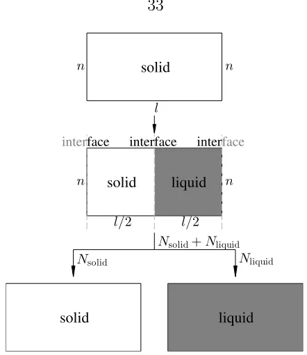
solid
l
n n
interface face
inter interface
solid liquid
l/2 l/2
n n
Nsolid+Nliquid Nsolid
solid
Nliquid
liquid
Figure 3.1: Schematic illustration of how the small-size coexistence method is exe-cuted in practice. Starting from then×n×l supercell with atoms in their ideal solid positions, we heat and melt the right half to obtain solid-liquid coexistence configura-tions. Then many parallel N P T MD simulations (here a total ofN =Nsolid+Nliquid) are performed in order to measure the probability distribution.
0 50 100 150
−7.2 −7.1 −7 −6.9 −6.8
t/ ps
H
/
eV
(a)
3100 3200 3300 3400 3500 3600 −7.3 −7.2 −7.1 −7 −6.9 −6.8 −6.7
12×6×6
averageH(single tra jectory)
Hlinearfit of solid/liquid
Tm=3325±1 K,lx=0.36±0.01
T/ K
H
/
eV
[image:46.612.212.433.55.310.2](b)