Data Collection and Distribution in Sensory Networks

Networks

Thesis by

C´edric Florens

In Partial Fulfillment of the Requirements for the Degree of

Doctor of Philosophy

California Institute of Technology Pasadena, California

2004

c

2004

Acknowledgements

I would like to begin by expressing my deepest gratitude to my advisor, Prof. Robert J. McEliece for his continuous guidance and support throughout my stay at Caltech. His sharp insight and infectious enthusiasm proved to be of inestimable value in my research endeavors and in the production of this document.

I would like to thank Prof. Robert J. McEliece, Prof. Jehoshua (Shuki) Bruck, Prof. Babak Hassibi, Prof. Steven Low at Caltech, and Dr. Polly Estabrook at the Jet Propulsion Laboratory for serving on my candidacy and defense committees, and for their advice on this thesis.

I am also indebted to Dr. Loren Clare and Dr. Jay Gao at the Jet Propulsion Laboratory for their encouragement and comments on my work.

I am grateful to my officemates Amir Dana, Radhika Gowaikar, Ravi Palanki, Chaitanya Rao, Masoud Sharif, Mihailo Stojnic and Jeremy Thorpe for making the Posner Communication Lab a pleasant and productive environment.

Abstract

The deployment of large-scale, low-cost, low-power, multifunctional sensory networks brings forward numerous and diverse research challenges. Critical to the design of systems that must operate under extreme resource constraints, the understanding of the fundamental performance limits of sensory networks is a research topic of particular importance. This thesis examines, in this respect, an essential function of sensory networks, viz., data collection, that is, the aggregation at the user location of information gathered by sensor nodes.

In the first part of this dissertation we study, via simple discrete mathematical models, the time performance of the data collection and data distribution tasks in sensory networks. Specifically, we derive the minimum delay in collecting sensor data for networks of various topologies such as line, multi-line, tree and give corresponding optimal scheduling strategies assuming that the amount of data observed at each node is finite and known at the beginning of the data collection phase. Furthermore, we bound the data collection time on general graph networks.

Contents

Acknowledgements iii

Abstract iv

1 Introduction 1

1.1 Sensory Networks: A Brief Overview . . . 1

1.2 Contributions . . . 4

1.3 Thesis Outline . . . 5

2 Deterministic Sensory Networks 6 2.1 Model and Problem Statement . . . 6

2.2 Directional Antenna Systems . . . 9

2.2.1 Line Networks . . . 10

2.2.2 Toward More General Scenarios . . . 14

2.2.3 Synchronization Problem . . . 19

2.2.4 2-line Networks . . . 20

2.2.5 Multi-line Networks . . . 22

2.2.6 Tree Networks, Case Where Base Station Degree Is 1 . . . 27

2.2.7 Tree Sensor Networks, General Case . . . 29

2.2.8 Networks with Cycles . . . 30

2.3 Omnidirectional Antenna Systems . . . 31

2.3.1 Line Networks . . . 31

2.3.2 Multi-line Networks . . . 35

2.3.3 Tree Networks, Case Where Base Station Degree Is 1 . . . 36

2.3.4 Tree Networks . . . 39

2.4 Omnidirectional/Directional Antenna Systems Comparison . . . 43

2.5 Conclusion . . . 44

3 Random Sensory Networks 46 3.1 Random Line Networks . . . 46

3.1.1 The Distribution of the Delay . . . 47

3.1.2 Asymptotic Analysis of the Average Delay . . . 49

3.1.3 Collected Data Distribution . . . 53

3.1.4 Multihop Case . . . 55

3.1.5 Packet Splitting to Improve the Average Delay . . . 57

3.1.6 A Simple Distributed Suboptimal Strategy . . . 58

3.1.7 Noisy Channel . . . 60

3.2 Random Multi-line Networks . . . 63

3.2.1 Delay Analysis for More General Topologies . . . 68

3.3 Comparison of Omnidirectional and Directional Systems . . . 69

3.3.1 Delay Distribution . . . 70

3.3.2 Asymptotic Analysis of the Average Delay . . . 71

3.3.3 Multi-line/Omnidirectional Case . . . 78

3.4 Dynamic Data Collection in Linear Sensor Networks . . . 81

3.5 Conclusion . . . 83

4 Conclusions and Future Directions 85

A A Preliminary Result 87

B Algorithms 90

List of Figures

1.1 Sensor node architecture. . . 1

1.2 Sensor nodes scattered in field. . . 2

1.3 Sensory network protocol stack. . . 4

2.1 Sensor nodes, gathered data, and sensor field. . . 7

2.2 Interference model parameters. . . 8

2.3 Sensory network. . . 9

2.4 Optimal distribution and collection schedules in 8-node line network. 11 2.5 (n+ 1)-node line network where r0 _{= 2r. . . . 14}

2.6 Minimum length data distribution schedule in 10-node line network with maximum transmission range of 3 hops. . . 19

2.7 Distribution schedules in synchronized and unsynchronized line network. . . 20

2.8 Worst-case out-of-sync distribution schedule in line network. . . 21

2.9 Optimal distribution schedule in 2-line sensor network. . . 21

2.10 Optimal distribution schedule for BS in 4-line sensor network. . . 23

2.11 “Equivalent” network construction. Distribution schedules in network N (solid arrows) and corresponding equivalent network Ne (solid ar-rows + dashed arar-rows). . . 24

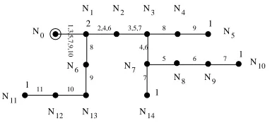
2.12 A 15-node tree network with degree of BS=1, the equivalent linear network is drawn in Fig. 2.4. Transmission time steps are written next to the edges. . . 27

2.13 Optimal distribution and collection schedules in 10-node line network equipped with omnidirectional antennas. . . 32

2.15 Optimal distribution schedules for BS in 2-line sensor network. Simple receive and forward sensor nodes on the right versus store and forward

nodes on the left. . . 37

2.16 A 16-node tree network whose BS degree is 1, the equivalent linear network is drawn in Fig. 2.13. Transmission time steps are written next to the edges. . . 37

2.17 5-node sensor network. . . 39

2.18 Network with cycles. To(G) = 10 TS, To(_TSP) = 18 TS. . . 42

2.19 Network with cycles. To(G) = 3 TS, To(_TSP) = 2 TS. . . 42

2.20 Network with cycles. To(G) =To(_TSP) = 18 TS. . . 43

3.1 Distribution of data collection time in 40-sensor node line network. Each sensor node carries 0 or 1 data packet with probability 1/2. . . 48

3.2 Distribution of data collection time in 40-sensor node line network. Each node in the considered network carries 0 or 1 data packet with probability 0.8 and 0.2 respectively. . . 49

3.3 Average collection time as a function of average number of packets per node and number of nodes in line network. Nodes carry 0 or 1 data packet with probability 1₋µand µrespectively. . . 54

3.4 Average collection time as a function of average number of packets per node in 500-node line network. Nodes carry 0 or 1 data packet with probability 1₋µand µrespectively. . . 55

3.5 Suboptimal distributed data collection strategy. . . 59

3.6 Data collection in line network under the assumption of an erasure channel. An erased packet is marked with a cross. . . 61

3.7 Ratio T_T(₍₀₎p) as a function of pin line network. . . 63

3.9 Difference between expected delay and average number of packets in network as a function of average number of packets per node and num-ber of lines in multi-line network (25 nodes per line). Nodes carry 0 or 1 data packet with probability 1₋µand µ respectively. . . 67 3.10 Distribution of data collection time in 40-sensor node line network.

Nodes carry 0 or 1 data packet with probability 0.7 and 0.3 respectively. 72 3.11 Average collection time as a function of average number of packets per

node and number of nodes in line network equipped with omnidirec-tional antennas. Nodes carry 0 or 1 packet with probability 1₋µand µrespectively. . . 76 3.12 Average collection time as a function of average number of packets per

node in 1500-node line network equipped with omnidirectional anten-nas. Nodes carry 0 or 1 packet with probability 1₋µandµrespectively. 77 3.13 Omnidirectional Line Network, ν _{∈ {}0,1_},E_{(T)−n0Lµ as a function}

of L and µ. . . 81 4.1 Optimal distribution schedule with respect to time that is suboptimal

with respect to energy. . . 86 4.2 Optimal schedule with respect to time and energy. . . 86 A.1 Optimal distribution schedule for BS in line network equipped with

List of Tables

Chapter 1

Introduction

In this chapter we give a brief overview of sensory networks main characteristics, applications, and research issues. The emphasis is put on the research topics relevant to the contents of this thesis. We summarize the main contributions of our work and conclude by an outline of this dissertation.

1.1

Sensory Networks: A Brief Overview

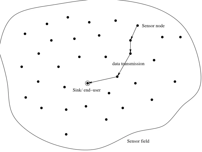
Recent technological advances in the Very Large Scale Integration (VLSI) field have contributed much to the development of microsensor systems. These combine vari-ous sensors, signal processing capabilities, data storage capabilities, wireless (radio, infrared or optical) communication capabilities, and energy sources on a single chip [1, 2, 43]. Such computational devices are referred to as sensor nodes and a collection of sensor nodes, possibly distributed over a wide area, connected through the wireless medium, form a sensory network. Fig. 1.1 illustrates the architecture of a sensor node while Fig. 1.2 illustrates a sensory network in a sensor field.

Memory

Processor Transceiver ADC

Power Sensors

Figure 1.1: Sensor node architecture.

[53, 20, 21]. Potential applications for such networks are numerous and can be broadly divided into military and civilian categories. Military applications include space ex-ploration [41], battlefield surveillance and enemy tracking [54]. Civilian applications include habitat monitoring [46, 10], environmental observation and forecast [68, 45], as well as various health applications [61].

Sensor field Sink/ end−user

Sensor node

data transmission

Figure 1.2: Sensor nodes scattered in field.

Sensor networks are wireless networks with unique characteristics which distin-guishes them from traditional wireless networks [69]. They are designed for unat-tended operation, must accommodate a traffic of statistical nature, support very low data rates to the order of 1-100 kb/s, and are characterized by a predominantly unidi-rectional flow of data from sensor nodes to sink. Sensory networks are members of the wireless ad hoc network family, that is, they are infrastructure-less networks unlike cellular networks. But they also distinguish themselves from MANETs1_{, designed to}

provide good throughput/delay characteristics under high mobility conditions, with-out much regard for energy consumption. Indeed, operation under severe constraints (lack of accessibility, limited energy resources and capabilities of nodes, absence of

infrastructure), not existent in more traditional networks, imposes aggressive en-ergy management [58]. Accordingly, in many sensor network applications, enen-ergy (or equivalently lifetime) is traded against throughput/delay. Finally, it should be noted that in a sensory network, while each node may be mobile, it is typically the case that once the target site of the particular sensing application is reached a semi-permanent stationary configuration is adopted for the purpose of gathering information. Accord-ingly the deployment of sensory networks brings forward numerous research problems [4, 70, 52].

network fundamental performance limits, and hardware design [57, 11, 49, 71].

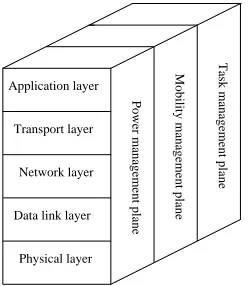
Application layer Transport layer

Network layer

Physical layer Data link layer

Power management plane

Mobility management plane Task management plane

Figure 1.3: Sensory network protocol stack.

1.2

Contributions

data-gathering sensory networks. Specifically, we derive, via simple discrete mathe-matical models, lower bounds on data collection time (delay) in data gathering sensory networks and exhibit algorithms that achieve those bounds [22, 23, 24, 25, 26, 27]. Most relevant to our research is the so-called packet routing problem which consists in moving packets of data from one location to another as quickly as possible in a network and has been studied in [44, 28, 29, 12, 9] with respect to wireline networks and general purpose wireless networks.

1.3

Thesis Outline

This dissertation is organized as follows: This chapter reviews briefly research issues in sensory networks and summarizes our contribution to the field. In Chapter 2, we describe optimal strategies to perform data collection under various assumptions and derive corresponding time performances with respect to a simple discrete mathemat-ical model for a sensor network. In this model the amount of data accumulated at each sensor node (characterized by a number of unit data packets) after some given observation period is assumed finite and determined. In typical scenarios however the exact amount of data accumulated at each sensor node is unknown which motivates the more complex model of the following chapter.

In Chapter 3, we model the number of data packets as a random variable and analyze the delay (which is now a random variable) in collecting sensor data at the base station. More specifically, we derive the distribution and the expected value of the delay for a line network using the optimal scheduling. Furthermore, we look into the effect of various parameters including size of packet, transmission range, and channel erasure probability on delay. We also propose a simple distributed scheduling strategy and analyze its delay performance showing that it is asymptotically optimal. Finally we extend our result to more general topologies such as multi-line networks and trees.

Chapter 2

Deterministic Sensory

Networks

In this chapter we study, with respect to a simple discrete mathematical model, the data collection problem in sensory networks. In this model, the amount of data accu-mulated at each sensor node (characterized by a number of unit data packets), after some given observation period, is assumed finite and determined. We refer to this net-work model as deterministic sensory netnet-work. More specifically, we describe optimal strategies to perform data collection and derive corresponding time performances.

This chapter is organized as follows: In section 2.1 we describe our sensor network model. We present results in deterministic sensory networks equipped with direc-tional antenna elements in section 2.2. In section 2.3, we propose a generalization to omnidirectional systems. We present a comparison analysis of the two systems in section 2.4. Finally, we conclude in section 2.5. Miscellaneous derivations for the chapter and Pseudo-code of presented algorithms are grouped in the appendices.

2.1

Model and Problem Statement

In this section, we describe the sensor network model on which the subsequent analysis is based and formulate our problem within the framework of this model. As noted in the introduction, in most sensing applications sensor nodes adopt a stationary configuration while information is being gathered. Correspondingly, our models will be static.

located within the sensor network (we refer to this node as the base station (BS) of the sensor network). In this chapter, we investigate the efficiency limits with respect to time of such data transfers.

We define a sensor network as a collection of n identical nodes_{N1, ..., Nn}. Each

node Ni is associated with an integer νi that represents the number of data packets collected by this node during the observation phase. N0 denotes the BS which is

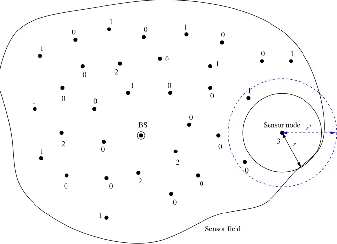
located within the network. Nodes (BS included) have limited wireless communica-tions capabilities and cannot receive and transmit at the same time. All the nodes including the base station have a common transmission rangerand interference range r0 _{(to be defined shortly). Fig. 2.1 illustrates sensor nodes, together with gathered}

data, scattered in a sensor field.

BS 0

1

0 1

0

0 1

1 0

2 0 1

0

1 0

1 0

0 1

3 0

0

0

0 2

2

0 0

2 1

0 0

1

r’

r

Sensor node

Sensor field

Figure 2.1: Sensor nodes, gathered data, and sensor field.

The interference model as defined in [34] for omnidirectional antenna systems is adopted here. That is, a transmission from node Ni to node Nj where i, j _≥ 0 is successful, if for every other node Nk, k_≥0 simultaneously transmitting

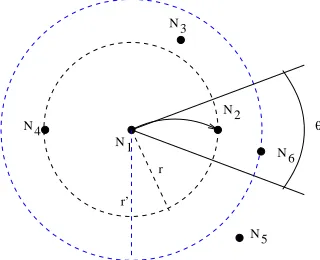
The second inequality specifies that node Nj must be outside the interference range of nodeNk and defines the interference region of nodeNkas the disc of radius r(1 +δ) centered at Nk. In directional antenna systems, on the other hand, the interference region of node Nk is only a portion of that disc, the sector formed by some angle θ. Fig. 2.2 illustrates the characteristic parameters of the model: sensor nodesN1, ..., N6,

the transmission range r and the interference range r0 _{= r(1 +δ). In directional}

antenna systems a transmission fromN1 toN2 creates interference at nodeN6 (inside

the sector formed byθ). However the same transmission creates interference at nodes N6, N3 and is received by nodeN4 (which is interference from the point of view ofN4)

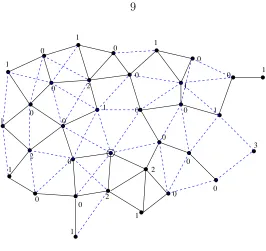
in omnidirectional antenna systems. Fig. 2.3 illustrates the sensory network formed by the nodes of Fig. 2.1. Nodes within transmission range are connected through a solid line while nodes within interference range are connected through a solid line or dotted line.

N 1 N 3

N 4

N 5 N 2 r

r’

N 6

θ

Figure 2.2: Interference model parameters.

We assume in our model that time is slotted and a one-hop transmission consumes one time slot (TS). The network is further assumed to be synchronous. A node can only transmit/receive one data packet per time slot. Multiple transmissions may occur within the network in one TS under this interference model by virtue of spatial separation. Such a network may be represented by a weighted rooted graph_{V, E,νn}

whereV =_{N0, ..., Nn},E denotes the set of links andνn= (ν₁, ..., νn). In this graph

1 2

0

1 0

2

1

1 0 1

2 1

0

1

0

0

0

0 0

0

1

3 0

1 0

1

1

2

0 0 0

0

0

Figure 2.3: Sensory network.

connection between two sensor nodes, or a sensor node and the BS. Thedata collection problem in a given sensory network is defined as the problem of routing all the data collected by the sensor nodes to the BS as efficiently as possible with respect to time and energy. The data distribution problem, on the other hand, is the problem of routing data to sensor nodes in a timely and energy efficient manner. In the following work we shall focus on the time efficiency alone of the data collection and distribution tasks.

2.2

Directional Antenna Systems

2.2.1

Line Networks

In this subsection, we consider a line network (an example of which is given in Fig. 2.4). A BS is placed at one end of the network. We assume sensor nodes are regularly placed along the network. We denote by d the distance between any 2 nodes. Assume each node is equipped with directional antennas allowing trans-missions over a distance r where d < r < 2d. Further assume that δ is such that (1 +δ)r < 2d. In this scenario there are two nodes (one on the left, one on the right) within transmission/interference range of any given node in the line (except for the end nodes). It is possible to extend this model to a more realistic scenario where nodes are randomly placed along a line and where different values of r, δ are considered (as long as end-to-end connectivity of the network is ensured). However, we find that simple case to be most insightful. In the following section, we consider more general scenarios. LetNi be the node at distance i from the BS. We denote by i _→ i+ 1 a transmission from node i to node i+ 1. Our goal is to determine the minimal duration of the collection phase and an associated optimal communication strategy.

For purpose of solving this problem we look initially at the following converse problem (which we shall refer to as thedistribution problem); instead of nodes sending packets to the BS, assume the BS is to transmit packets to nodes. The data transfer efficiency remains our concern. This problem is of separate interest in sensor networks.

We propose the following simple algorithm for solving the distribution problem. We shall prove subsequently it is optimal. The BS is to send first data packets destined for the furthest node, then data packets for the second furthest one and so on, as fast as possible, while respecting the channel reuse constraints. Nodes between the BS and its destinations are required to forward packets as soon as they arrive (that is in the TS following their arrival). We include, in Appendix B, Algorithm 1 running at the BS.

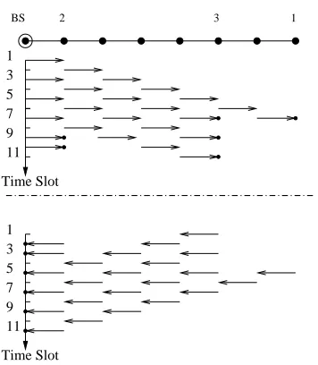
The procedure is illustrated on an example, where V =_{0,1,2,3,4,5,6,7_},E =

The schedule of transmissions, as determined by Algorithm 1, is drawn below the network for the distribution and collection problems respectively. Either way it is performed in 11 TS.

2 3 1

1 3 5 7 9

1 3 5 7 9 11 11

Time Slot

Time Slot

BS

Figure 2.4: Optimal distribution and collection schedules in 8-node line network.

Next we determine the performance of our algorithm in general. Denote by Ti the last busy TS at node iin the execution of our distribution algorithm (In the previous example, we have T1 = 10, T2 = 9, T3 = 10, T4 = 11, T5 = 11, T6 = 7, T7 = 7). Clearly

then our algorithm runs in max

1≤i≤n{T i}. Ti is a function of the distance to the BS, the number of packets destined for node ias well as the number of packets forwarded by nodei. Assuming νi = 0 for i > n, node i’s last busy TS when running Algorithm 1 is

Ti =       

     

i₋1 + 2P_j≥i+1νj if νi = 0

ν1+ 2Pj≥2νj if i= 1 and ν1 ≥1

i₋2 + 2P_j≥iνj if i_≥2 and νi _≥1

(2.2)

a data packet consists in receiving that data packet and transmitting it right away and therefore a node involved in forwarding one data packet will remain busy two consecutive TS. Receiving a data packet on the other hand consumes only one TS but in our scheme forces node i_≥2 to remain silent in the following TS. Therefore,

ν1 ≥1⇒T1 = 2

X

j≥2

νj+ν1

νi _≥1, i >1_⇒Ti = (i₋1) + 2 X j≥i+1

νj + 2(νi₋1) + 1

νi = 0_⇒Ti = (i₋1) + 2 X j≥i+1

νj

We define, for a given sensor network, Tu(ν) the minimum length of a time schedule

over all time schedules that perform the distribution job.

Theorem 2.2.1. Assuming νi = 0 fori > n, the minimal data collection time in the

directional line network ν of length n1 is

Tu(ν) = max

1≤i≤n−1(i−1 +νi+ 2

n X

j≥i+1

νj) (2.3)

Proof. Clearly the maximum ofTi is obtained over the set _{i_≥1_|νi ₆= 0_}. Thus we have the following upper bound onTu(ν)

Tu(ν)≤ max

{i≥1|νi6=0}Ti

A lower bound on Tu(ν) is as follows. Assuming νi = 0 for i > n, we have

Tu(ν)≥ max

1≤i≤n−1(i−1 +νi+ 2

n X

j≥i+1

νj)

Indeed node i has to forward Pn_j≥i+1νi data packets to further nodes. Forwarding one data packet consists in receiving and transmitting that data packet and therefore

results in a two TS consumption (per forwarded packet). Besides, it is itself the destination of νi data packets. Each received data packet costs at least one TS. Furthermore, node i can’t be active before it receives a data packet, which takes at leasti₋1 TS. Therefore,Si ,2P_j≥i+1νj+νi+ (i₋1) is a lower bound on any time schedule for all i. Hence, max

1≤i≤n−1Si is a lower bound onTu(ν).

Finally, we prove that lower and upper bounds on Tu(ν) are equal and therefore

the proposed schedule is optimal: Clearly S1 =T1 and ∀i ≥2, Si =Ti if νi ≤1. On

the other hand, ifνi >1 then Ti > Si but then either νi−1 = 0 and then Si−1 =Ti or

νi−1 ≥1 and then Si−1 > Ti.

Corollary 2.2.2. In the particular case where no two consecutive components of

vector ν equal zero, Eq. (2.3) reduces to:

Tu(ν) = ν1 + 2

X

i≥2

νi (2.4)

We now return to the data collection problem. The construction of a schedule here is based on the symmetry of the operations of distribution and collection. A time schedule that is symmetric to the distribution problem’s schedule with respect to a fictive horizontal axis (see example in Fig. 2.4) provides us with an optimal solution, the time to transmit data packets from nodes to the BS being the same as the time to carry out the converse operation (and being therefore minimal). In particular a transmissioni_→i+ 1 occurring at TSj in the distribution problem is a transmission i+ 1_→i occurring at TSTu(ν) + 1−j in the collection problem. Since the solution

2.2.2

Toward More General Scenarios

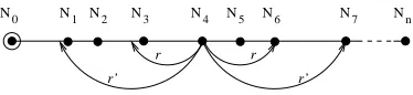
The general line case is shown in Fig. 2.5. It consists of n randomly located sen-sor nodes N1, . . . , Nn along a line and a BS N0 at the left end of that line. It is

assumed that each node’s transceiver has a common transmission range r such that r_≥ max

0≤i≤n−1d(Ni, Ni+1) where d(Ni, Ni+1) denotes the distance between nodesNi and

Ni+1 (which ensures end to end connectivity of the network) and interference range

r0 _{= (1 +δ)r. Under these assumptions any given node will have in general more that}

one neighbor to the right (resp. left), those numbers varying from one node to the other. Particular cases of this scenario are solved in the remaining of this section. We first study the case where the transmission range is fixed and equal to one hop and the interference range is variable. We then study the case of variable transmission range.

r r

r’

N₁ N₂ N₃ N₄ N₅ N₆ N₇ N_n N₀

r’

Figure 2.5: (n+ 1)-node line network where r0 _{= 2r.}

This analysis constitutes a generalization of the line network analysis in the previ-ous section which allows us to study the respective impact of the transmission range and the interference range on the data collection process. We assume, for simplicity, that the number of left and right neighbors is the same (one in this case) for all nodes. Furthermore, it is convenient to imagine a line network with regularly spaced sensor nodes.

First case: variable interference range

We fix the transmission range to 1 hop and the interference range tom hops (that is r = 1 and δ = m₋1). Note that in the previous section, m was taken to be 1. In practice m is often between 2 and 3.

reuse/transceiver constraints. This strategy’s time performance is max

i Ti where

T1 =

                  

Pm−1

1≤j jνj +m

P

j≥mνj if ν1 ≥1

2 +m(P_j≥mνj₋1) if _∃k_≥m such that: ν1 =. . .=νk−1 = 0, νk ≥1

2 +k(νk₋1) +Pm_k+1≤−1 _jjνj+mP_j≥mνj if

∃k2_≤k < m, ν1 =. . .=νk−1 = 0, νk≥1

T2 =

                   P

2≤j≤m−1jνj+m

P

j≥mνj if ν2 ≥1

3 +m(P_j≥mνj₋1) if _∃k_≥m such that: ν2 =. . .=νk−1 = 0, νk ≥1

3 +k(νk₋1) +Pm_j≥−1_k+1jνj+mP_j≥mνj if

∃k2_≤k < m, ν2 =. . .=νk−1 = 0, νk≥1

Ti = X i≤j≤m−1

jνj +mX j≥m

νj if 2< i < m

Tm+k =   

 

k+mP_j≥m+kνj if νm+k≥1 k+ 1 +mP_j≥m+kνj if νm+k = 0

if k_≥0

The proof follows a similar argument as the one used to prove Eq. (2.2) and is omitted. The following theorem gives a closed form expression for the minimum data collection delay. This generalizes Theorem 2.2.1.

Theorem 2.2.3. The minimum data collection time Tm

u (ν) on directional line

net-work ν, when the transmission range is 1 hop, and the interference range is m hops,

is

T_um(ν) =

     max

i (i−1 +

Pi+m−2

j≥i (j−i+ 1)νj +m P

j≥i+m−1νj, ∀m≥2

max

i (i−1 +νi + 2 P

j≥i+1νj) if m = 1

(2.5)

Proof. We have Tm

u (ν)≤max

can be derived as well.

∀i_≥1, T_um(ν)≥i−1 +

X

j≥i

νj + X j≥i+1

νj+. . .+ X j≥i+m−1

νj (2.6)

Indeed transmissions i₋1_→i, i_→i+ 1, . . . , i+m₋2_→i+m₋1 may not occur concurrently due to channel reuse constraints. Inequality (2.6) may be rewritten

∀m _≥2, T_um(ν)≥max

i (Si) (2.7)

where

Si ,(i₋1 + X i≤j≤i+m−2

(j₋i+ 1)νj +m X j≥i+m−1

νj) (2.8)

The case m = 1 may be derived from the above formula by choosing m = 2. Assume there exists j0, 1≤j0 ≤n such that∀i6=j0, Tj0 ≥Ti Tj0+1 < Tj0

• if j0 = 1 then ν1 ≥1⇒S1 =T1

• if j0 = 2 then ν2 ≥1, ν1 = 0⇒T2−S2 =P_2≤j≤mνj −1≥0

ν1 = 0⇒T1 =T2 ⇒S1 ≥T2. Indeed S1 ≥T1 since

ν1 ≥1⇒S1 =T1

and ν1 = 0⇒S1 −T1 =

  

 

P

1≤j≤m−1jνj +m−2≥0 (m≥2) or

P

1≤j≤k−1jνj +k−2≥0 (k≥2)

• if 2< j0 < m⇒νi ≥1, ν1 =. . .=νi−1 = 0⇒Tj0 −S1 =−P_{1≤j≤i−1}jνj = 0

• if j0 =m+k k ≥ 0 ⇒νm+k ≥1 νk =. . . =νk+m−1 = 0 ⇒ Tm+k−Sk+1 = −Pkj≥+km+1−1(j−k)νj = 0

Therefore max

Second case: variable transmission range

In this section, we consider the problem of scheduling when each node is allowed to use up to h hops. Of course, a longer transmission range leads to faster data collection. This is quantified in the following theorem where the minimum data collection time Tmin(h,νn) is expressed as a function of the transmission range h (hops).

Theorem 2.2.4. For a one-sided line network of length n in which theith node has

νi packets and is equipped with directional antennas, the minimum collection time of

the packets at the BS as a function of the transmission range h in hops is

Tmin(h,νn) = max(S0, S1, S2, . . . , Sn−h) (2.9)

where

Si = n X

j>i+h νj +

$ Pn

j>i+hνj−1 + (i modh) h

%

+

i h

+ 1, 0_≤i_≤n₋h

S0 _{= S}

0 + max

l X

j=1

νj −1,0 !

+ h X

j=l+1

νj (2.10)

where l is the unique solution to l+n0 = 0 mod h such that 0≤l≤h−1. Remark: Note that when h= 1, Eq. (2.9) reduces to the familiar Eq. (2.3).

Proof. The proof is similar to the proof of the case h = 1. Here we only outline the generalization. The proof has two parts. Firstly, we need to show that the right-hand side of (2.9) is a lower bound for the collection time. Secondly, we prove it is an upper bound as well by exhibiting a schedule with this time performance.

In order to show that the right-hand side is a lower bound, we first consider the h nodes i,1_≤ i_≤ h closest to the BS. They need to forward nh =P_j>hνj packets. If nh ≤ h, this can be done in nh + 1 TS or more. This takes exactly nh + 1 TS if all packets to be distributed are located at node h+ 1 and more otherwise. If h+ 1 _≤ nh ≤ 2h, this can be done in nh+ 2 TS or more. So in general it takes at least nh +_bnh−1

forwarded by the h nodes j, i+ 1_≤ j _≤ i+h, it can be shown that it takes at least

ni,h+_bni,h+(ni,h modh)−1

h c+b i

hc+1 TS to do so. Therefore the maximum of the previous expression overigives a lower bound for the data collection time performance. We are not done though. Indeed this lower bound is not achievable when there are packets to be distributed at distanceiwhere i,1_≤i_≤h. An additional lower bound may be derived to handle this case by reconsidering the first h nodes. They must not only forward P_j>hνj packets, but also receive P_j≤hνj packets. The lower bound S0 may

be adjusted (to S0_{) to take this fact into account.}

A possible (optimal) schedule for the distribution problem is as follows. It consists of transmitting data packets first to the furthest node, then to the second furthest node and so on as fast as possible until all packets at distance greater than h have been served. Packets at distance i,1 _≤ i _≤ h are served in the reversed order, i.e, from closest to the BS to furthest. To prove this is indeed optimal, we compute the algorithm’s time performance and show it achieves the lower bound previously exhibited. This is similar to what was done in the case h= 1 and is left out here for the sake of brevity.

In order to get a better insight into the result of Theorem 2.2.4, we give a simple illustrative example.

Example: We consider a line network of length n, where each node carries exactly one data packet and has a transmission range of h _≤ n hops. Direct application of Theorem 2.2.4 gives the minimum collection time as

T =n+_bn

hc −1 (2.11)

BS 1 1 1 1 1 1 1 1 1 1 1

3 5 7 9 11 13

Figure 2.6: Minimum length data distribution schedule in 10-node line network with maximum transmission range of 3 hops.

2.2.3

Synchronization Problem

Up to now we have assumed that all sensor nodes and BS were synchronized. In this section, we study the impact on the data collection time of lack of synchronization in the network. In our communication model we have assumed that the transmission of a data packet consumed one TS. Let us be more precise. The transmission of a data packet is made up of a transmission phase (at the transmitting node), a propagation phase (from the transmitting node to the receiving node) and a reception phase (at the receiving node). Assuming sensor nodes are about one meter apart, that the size of a data packet is about 20 bytes and data rates are of the order of 10 kbps, we can get an idea of the duration of each phase. We find ∆T X = ∆RX = 1.6_∗10−2 _s

which is very large compared to the propagation time 0.33_∗10−8 _{s. The latter may}

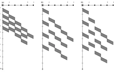
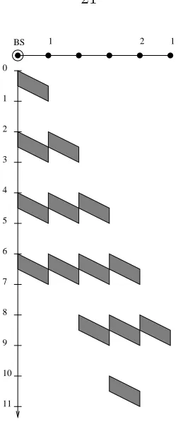
therefore be ignored for the purpose of this analysis. Then, the first half of the TS is used for transmission of the data packet at the transmitting node while the second half is used for reception of the data packet, by the receiving node. Fig. 2.7 illustrates the distribution schedule for a particular network assuming perfect synchronization (left figure, delay is 6 TS) and multiple unsynchronized cases. In the middle figure all sensor nodes are synchronized but out-of-synch with the BS and the delay is 8.5 TS. In the right figure the sensor node at distance one from the BS is out of synch with other nodes and the delay is 9 TS. We have the following theorem.

line network is

Tus(ν) = max

1≤i≤n−1(2i−3 +νi+ 2

n X

j≥i+1

νj) (2.12)

Proof. The proof follows a similar argument as the one used to prove Theorem 2.2.1.

The worst-case performance for the previous example is illustrated in Fig. 2.8. Delay becomes 11 TS. In conclusion the data collection time is quite sensitive to variation in clock synchronization. Our analysis shows indeed worst-case performance degradation in the order of 50 %.

BS 1 2 1 BS 1 2 1 BS 1 2 1

1 2 0

3 4 5 6 7 8 9 10

Figure 2.7: Distribution schedules in synchronized and unsynchronized linenetwork.

2.2.4

2-line Networks

Consider now a line network and place the BS anywhere on that line. This may be seen as a 2-line network (µ,ν). We denote by Tu(µ,ν,) the optimal performance

BS 1 2 1

1 2 0

3 4 5 6 7 8 9 10 11

Figure 2.8: Worst-case out-of-sync distribution schedule in line network.

multi-line algorithm described in the next section, is illustrated in the example of Fig. 2.9.

1 2

2 1 3

Time Slot 9 11

7 5 3 1 1

Figure 2.9: Optimal distribution schedule in 2-line sensor network.

is

Tu(µ,ν) =

  

 

max(Tu(ν) + 1,P_i≥1µi+νi) if Tu(µ) =Tu(ν)

max(Tu(ν),P_i≥1µi+νi) if Tu(ν)> Tu(µ)

(2.13)

Proof.

Tu(µ) =Tu(ν)⇒Tu(µ,ν)≥max(Tu(µ) + 1,

X

i≥1

µi+νi))

Tu(µ)> Tu(ν)⇒Tu(µ,ν)≥max(Tu(µ),

X

i≥1

µi+νi))

It is easy to see why the above described algorithm achieves this lower bound. Con-sider for example the case Tu(µ) = Tu(ν). Either the algorithm takes T(µ) + 1 TS

to perform the job or it takes T0

−1 (resp. T10) defined as the last busy TS at

dis-tance 1 to the left (resp. to the right) from the BS. If it so T0

−1 (resp. T10) equals

P

i≥1µi+νi).

2.2.5

Multi-line Networks

according to the following rule. If a legal direction was not chosen, its new estimate becomes its old estimate plus one. Illegal direction estimates remain unchanged. The idea is to minimize at each TS the overall estimate of the transmission time.

We illustrate the procedure on an example in Fig. 2.10. In the accompanying table, we list data transfer completion time estimates at each TS and the corresponding decision made by the BS. As previously stated the initial completion time estimates are computed using Eq. (2.3). The table reads as follows. TS 1: All 4 transmission directions are legal. The BS chooses to transmit toward lineA. At TS 2, transmitting toward A is not a legal move, the legal transmission direction associated with the biggest estimate is B, etc. Along a given line, the packets destined for furthest nodes are sent first by the BS. As for the other nodes they merely forward the data packets of which they are not recipients (a packet is transmitted in the following TS that it was received). In this example the algorithm performance is 10 TS.

3

(A)

(B)

2 1

1

1 9 7 5 3 A TS A B C D BS 2 9 8 6 4 B 3 9 8 7 5 A 4 9 8 8 6 B 5 9 8 9 7 A 6 8 10 8 C 7 9 9 B 8 10 D

(D)

1

(C)

Figure 2.10: Optimal distribution schedule for BS in 4-line sensor network.

Theorem 2.2.7. Algorithm 2 is optimal.

Proof. We note that equivalently this algorithm picks at each TS the legal direction Bi that maximizes T(νi) (that quantity being updated at each TS to take into

ac-count the packets delivered).

of scheduling data transfers to the nodes. Let P0 _{denote the same problem under a}

relaxed set of conditions, namely that simultaneous transmission and reception (of different data packets) are allowed in a single TS at any given node. This problem is independently studied in Appendix A. LetS(P, N) denote a schedule for problem P and network N. LetS|BS(P, N) denote the schedule of the BS derived fromS(P, N).

LetSopt_{(P, N) denote an optimal schedule for (P, N).}

In the “equivalent” network Ne of Network N the data packets along a particular line are redistributed along the corresponding line in Ne in the manner illustrated in Fig. 2.11.

2 1 1 1 ₁

BS 2 3 1

N e N

Figure 2.11: “Equivalent” network construction. Distribution schedules in network N (solid arrows) and corresponding equivalent network Ne (solid arrows + dashed arrows).

Although packets in N and Ne are distributed differently over the network, we shall see that the data collection is the same for both networks. It is in that sense that they are “equivalent.” Formally the construction is as follows. To each line of N, say Bk, ifνk

i denotes the number of data packets at distance ifrom the BS along Bk, T(νk) denotes the length of an optimal schedule for that particular line, andT_ik

i from the BS alongB0

k, then

i= 1 ν₁0k =ν₁k i_≥2 ν_T0k₍νk_)−Tk

i+2j+i = 1 f or 0≤j ≤l−1 if ν

k

i =l≥1 (2.14) ν_i0k = 0 otherwise

By construction, Ne has the following characteristics:

• Same total number of data packets asN, same number of data packets per line, same number of lines.

• Each line carries the same workload as its corresponding line in N (i.e., _∀k, T(ν0k) = T(νk)).

• Node i >1 carries 0 or 1 data packet.

• Two nodes with data packets are separated by at least one node with no data packet.

Example: Consider the following 2-line network N: B1 : ν1 = (0,4), B2 : ν2 =

(2,0). Its equivalent network Ne is a 2-line network such that: B0

1 :ν01 = (0,1,0,1,0,1,0,1),B20 :ν02 = (2,0) =ν2

Lemma 2.2.8. There exists an optimal schedule for problem P0 _{and network Ne.}

Proof. A construction of such a schedule is given in Appendix A.

Lemma 2.2.9. Let Sopt_(P0_{, Ne)denote the optimal schedule constructed in Appendix} A for problem P0 _{and network Ne. It is possible to construct a schedule S(P, Ne)}

for problem P and network Ne from Sopt_(P0_{, Ne) by judiciously reordering the BS} transmissions such that the two schedules have the same length.

Proof. With the convention that furthest nodes should be served first along a given line, a schedule S(P/P0_{, Ne) is entirely defined by its restriction to the BS schedule}

the lines toward which transmit at each TS as well as possible silences (correspond-ing to BS be(correspond-ing idle). S|BS(P0, Ne) = (B10, B10, B10, B10, B20, B20,−,−) is an instance of

an optimal schedule for problem P0 _{and the network described in previous example}

where “-” denotes a silence.

We construct S(P, Ne) from Sopt_(P0_{, Ne) by iteratively applying the following}

opera-tion on S: insert(i, j)(S) for j > i_≥ 1 which returns a schedule S0 _{where element j}

in schedule S was inserted between elementi andi+ 1 inS. In the previous example insert(1,5)(S|BS(P0, Ne)) = (B10, B20, B10, B10, B10, B20,−,−).

This operation doesn’t change the length of S, that is Length(S0_{) = Length(S) as}

long as it is not applied more than once for any i. This is a direct consequence of the fourth characteristic of an equivalent network. Next we describe the construction. IfS is a valid schedule (i.e., satisfying constraint P) we are done. Otherwise assume the first conflict occurs in position i0 of schedule S (that is constraint P does not

allow for transmission toward element i0 followed by transmission toward element

i0 + 1). In the instance above, there are conflicts in i0 = 1,2,3,5. Further assume

the first direction distinct from the one in position i0 and that follows it is element

i1 of S. If there is no such direction then denote i1 the position of the first silence

following (it always exists by definition of Ne). Then apply insert(i0, i1)(S). Clearly

the procedure produces a new schedule S of same length. Thus the portion of the schedule S comprised between element 1 and i0 + 1 satisfies P. Repeat until the

schedule S satisfies constraint P. Since the number of initial conflicts is finite, this procedure ends in a finite number of steps. In the previous example these operations are in order: insert(1,5), insert(3,6) and insert(5,7). They lead to the schedule: S|BS(P, Ne)) = (B10, B20, B10, B20, B10,−, B10,−)

By lemma 2.2.9, the lengths of S(P, Ne) and Sopt_(P0_{, Ne) are the same. Thus}

S(P, Ne) is optimal. Denote it Sopt_{(P, Ne). One may construct a schedule S(P, N)} fromSopt_{(P, Ne) such that the lengths of the two schedules are the same andS}

may construct a schedule S0_{(P, Ne) such that the two schedules have the same length}

and S0

|BS(P, Ne) = S|0BS(P, N) so the length of S0(P, Ne) is less than the length of Sopt_{(P, Ne), a contradiction. Thus S(P, N) is optimal, which concludes the proof of} Theorem 2.2.7.

2.2.6

Tree Networks, Case Where Base Station Degree Is 1

Throughout this paragraph we assume that the degree of the root of the consid-ered graphs is one. We define the equivalent linear network (Gl, El,νl) of a network

(G, E,ν): IfG={N0, N1, . . . , Nn}andν = (ν1, . . . , νn) thenGl={0,1, . . . , m}, El= {(i ₋1, i),1 _≤ i _≤ m_} and νl = (νl1, . . . , νlm) where m = max

i (d(N0, Ni)) and νlj = P_i|d(N0,Ni)=jνi We illustrate a tree network in Fig. 2.12 (n = 14, m = 7); its equivalent linear network is shown in Fig. 2.4.

1

1

8

9 10 11

7

1,3,5,7,9,10

2,4,6 3,5,7 8 9

5 6

4,6

7

1

1

2 N₀

N₁ N₂ N₃ N₄

N₅ N₆

N₁₁

N N N₇

N₈ N₉ N

N

12 13

10

14

Figure 2.12: A 15-node tree network with degree of BS=1, the equivalent linear network is drawn in Fig. 2.4. Transmission time steps are written next to the edges.

The equivalent linear network’s schedule may serve as a schedule for the initial tree network. Next we explain how transmission time slots for (Gl, El,νl)

(deter-mined by running algorithm 1) may be mapped onto (G, E,ν). Consider an element

Pα = {P | ∃e ∈Eα ∩path(P)}. We define Tα = {TS used by (α, α+ 1) ∈ El}. We have _|Pα| = P

(Ni,Nj)∈Eα

(νj +fj) =P k>α

νlk =_|Tα|. Thus one may define a one-to-one correspondence g between Pα and Tα that associates the packet P with the longest path in Pα, with the TS with the smallest index in Tα; the packet P with sec-ond longest path, with the TS with secsec-ond smallest index and so on. We finally define P(Ni0,Nj0)

α ={P |(Ni0, Nj0) ∈ path(P)}⊆ Pα. (Ni0, Nj0) is associated with time slots g(P(Ni0,Nj0)

α ). In the example of Fig. 2.12, we have {P} ={P1,P2,. . . ,P6}

where the first packet is characterized by path(P1) = (N0,N1,N2,N3,N7,N8,N9,N10),

the second one by path(P2) = (N0,N1,N2,N3,N4,N5), the third one by path(P3) =

(N0,N1,N6,N13,N12,N11), the fourth one by path(P4) = (N0,N1,N2,N3,N7,N14), and

finally the fifth and sixth ones by path(P5) =path(P6) =(N0,N1). We also have E1 = {(N1,N2),(N1,N6)},P1 ={P1,P2,P3,P4},T1 ={2,4,6,8}, and P1(N1,N2) ={P1,P2,P4}.

Thus edge (N1,N2) is associated with time slots g(P(1N1,N2)) ={2,4,6}. Thus

Algo-rithm 1 run on the equivalent linear network provides a BS transmission schedule. Intermediate nodes simply forward data packets to further nodes as they arrive (in the TS following their arrival). This requires a routing table at junction nodes. In a centralized version of this algorithm nodes may be informed of their transmission slots. Fig. 2.12 shows such a mapping for the considered example.

Although an equivalent linear network has a reduced set of possible concurrent transmissions, this procedure produces an optimal transmission schedule. This follows from the following lemma.

Lemma 2.2.10. Given any connected graph Gsuch that degree of BS is one, if t2(G) denotes the time performance of a given data distribution algorithm, and νj denotes the number of data packets at distance j from the BS, then

t2(G)≥max

i (i−1 +νi+ 2 X

j>i

νj) (2.15)

but link (0,1) can not be activated at the same time as a link (1,2), thus we have t2(G)≥Pj≥1νj +

P j≥2νj.

P

j≥iνj data packets must be delivered to nodes at distance greater than i > 1. Therefore edge (0,1) is activated at least P_j≥iνj times and edges (1,2) P_j>iνj times but link (0,1) can not be activated at the same time as a link (1,2), moreover after P

j≥iνj + P

j>iνj TS the last data packet sent by the BS is at distance 0 or 1 from the BS if νi > 0 and at distance 0, 1 or 2 from the BS if νi = 0. Indeed it takes a minimum of 2P_j≥iνj TS to get all the data packets out of the positions 0,1,2. Thus afterP_j≥iνj+P_j>iνj TS whether νi >0 or νi = 0 one data packet is at leasti₋1 hops away from its destination, therefore: t2(G)≥Pj≥iνj +

P

j>iνj+i−1. Hence the stated result.

2.2.7

Tree Sensor Networks, General Case

The results in the previous sections suggest the following algorithm for dealing with general tree networks.

1. Linearize the subtrees attached to the BS (with BS degree equal to 1) according to the procedure described in section 2.2.6.

2. Apply multi-line algorithm described in section 2.2.5 to the resulting multi-line system.

This procedure produces an optimal schedule. This results from Theorem 2.2.7 and Lemma 2.2.10.

Theorem 2.2.11. If _T is a tree network and νk

j denotes the number of data packets

at distancej from the BS along branchk, then the minimum data collection time over

T is

Tu(T) = max

1≤i≤n(i−1 + n X

j≥i

ν_j0) (2.16)

where ν0

j = P

kνj0k and νj0k is obtained from νjk by equation (2.14).

2.2.8

Networks with Cycles

We propose a data distribution/collection strategy on general graphs. However that strategy is not optimal in general. In this section we prove that our algorithm performs within a factor of 2 of an optimal strategy. The proposed strategy consists of two subprocedures:

1. Extract a shortest path spanning tree _TSP.

2. Apply previously described distribution strategy on trees to _TSP.

Note: one can show that shortest path spanning trees always exist by using Dijkstra algorithm. The following theorem provides a motivation for choosing a shortest path spanning tree. The proof follows from Theorem 2.2.11.

Theorem 2.2.12. For any (connected) graph G, for any spanning tree _T of G and for any shortest path spanning tree _TSP of G, the minimum data collection time over

network _T, Tu(_T) satisfies

Tu(_TSP)≤Tu(T) (2.17)

Theorem 2.2.13. For any (connected) graph G, and any shortest path spanning tree TSP we have

Tu(TSP)

2 ≤Tu(G)≤Tu(TSP) (2.18)

Proof. The second inequality is clear. For a proof of the first inequality we define: t1(G) the minimum distribution time when transmission and reception are

simulta-neously allowed in a TS at any given node. Clearly t1(G) ≤ Tu(G). By corollary

A.0.4 we also have t1(G) =t1(TSP). Besides for any connected graph A the following inequality holds: Tu(A)_≤2t1(A). ChooseA=TSP, the inequality follows.

TSP is the line network ν = (

k−1

z }| {

0,0, ...,0, n). We have Tu(G) = n+k ₋1 (for k _≥ 1) and Tu(_TSP) = 2n+k−2 (for k ≥2), thusTu(G) converges toward Tu(TSP)/2 when n goes to infinity (for k_≥2).

Bounds on Tu(G) can also be written in the following more explicit way.

Theorem 2.2.14. The minimum data collection time over a graph G satisfies

max

i (i−1 + X

j≥i

νj)_≤Tu(G)_≤max

i (i−1 +νi+ 2 X

j≥i+1

νj) (2.19)

Proof. We have from corollary A.0.4 t1(G) = max

i (i−1 + P

j≥iνj)

Both bounds on Tu(G) are achievable. The lower bound for instance is achieved in the previously considered example where max

i (i−1 + P

j≥iνj) =n+k−1.

2.3

Omnidirectional Antenna Systems

Results on directional antenna systems may be to some extent adapted to omnidirec-tional antenna systems. This is the purpose of this section.

2.3.1

Line Networks

Our results readily extend to omnidirectional antenna systems. The procedure is illustrated in the example of Fig. 2.13 whereV =_{0,1,2,3,4,5,6,7,8,9_},E=_{(i, i+ 1),0_≤i_≤8_},ν = (2,1,0,0,0,0,0,1,1), d < r <2d, (1 +δ)r <2d.

The schedule of transmissions, as determined by Algorithm 3 in appendix B, is drawn below the network (upper schedule) for the distribution problem. It is performed in 11 TS.

Next we determine the performance of our algorithm in general. Denote Ti the last busy time slot at node i, 1_≤i_≤nin the execution of our distribution algorithm (In the previous example, we have T1 = 10, T2 = 8, T3 = 7, T4 = 8, T5 = 9, T6 = 10, T7 =

11, T8 = 11, T9 = 9). Clearly then our algorithm runs in max

1 3 5 7 9 11

1 1 1

1 3 5 7 9 11 Time Slot

Time Slot 2 BS

Figure 2.13: Optimal distribution and collection schedules in 10-node line network equipped with omnidirectional antennas.

of the distance to the BS, the number of data packets destined for nodei (that is νi) and the number of data packets forwarded by node i.

Assuming νi = 0 for i > n, we have

T1 =

  

 

3P_j≥3νj₋1 if ν1 = 0, ν2 = 0 and P_j≥3νj ≥1

ν1+ 2ν2+ 3P_j≥3νj otherwise

T2 = 2ν2+ 3

X

j≥3

νj

∀i_≥3

Ti =       

     

i₋2 + 3P_j>iνj if νi = 0 andP_j>iνj _≥1 i+ 3P_j>iνj if νi = 1

i₋3 + 3P_j≥iνj if νi _≥2

(2.20)

If i= 1,

ν1 = 0, ν2= 0, fi ≥1⇒Ti = 3(fi−1) + 2 + (i−1) otherwise, Ti =ν1+ 2ν2+ 3(fi−ν2)

If i= 2,

Ti = 2ν2+ 3(fi−ν2) ∀i_≥3,

νi = 0, fi_≥1_⇒Ti = 3(fi₋1) + 2 + (i₋1) ν1 ≥1⇒Ti = 3fi+ 1 + (i−1) νi _≥2_⇒Ti = 3fi+ 3(νi₋1) + 1 + (i₋1)

but,

fi =X j>i

νj

hence the stated result.

Clearly the maximum ofTi is obtained over the set _{i_≥1_|νi ₆= 0_}. We define, for a given sensor network, To(ν) the minimum length of a time schedule over all time

schedules that perform the distribution job. Thus we have the following result.

To(ν)≤ max

{i≥1|νi6=0}Ti (2.21)

Let’s now derive a lower bound on To(ν). Assuming νi = 0 for i > n, we have

To(ν)≥ max

1≤i≤n(i−1 +νi+ 2νi+1+ 3 X

j≥i+2

νj) (2.22)

Proof. Consider node i_≥1, assume there exists k_≥i such that νk _≥1. Then

• edge (i₋1, i) is activated P_j≥iνj TS.

• edge (i, i+ 1)-if it exists- is activated P_j≥i+1νj TS.

Clearly transmissions i₋1 _→ i, i _→ i+ 1, i+ 1 _→ i+ 2, _∀i _≥ 1 may not occur concurrently (channel reuse constraints). Besides from our initial assumptions we know that idle time of nodes _{∈ {}i, i+ 1, i+ 2_{} ≥}i₋1. Therefore,

To(ν)≥

X

j≥i

νj+ X j≥i+1

νj+ X j≥i+2

νj+ (i₋1),Si

We have _∀i, To(ν)≥Si, thus To(ν)≥max

i Si.

Next we prove that the lower bounds and upper bounds previously derived on To(p) are in fact equal and hence that the proposed schedule is optimal.

Theorem 2.3.1. Assuming νi = 0for i > n, we have that the minimum data collec-tion time, in the line network ν of lengthn2 equipped with omnidirectional antennas,

is

To(ν) = max

1≤i≤n(i−1 +νi+ 2νi+1+ 3 X

j≥i+2

νj) (2.23)

Proof. Assume there exists j such that _∀i₆=j, Tj _≥Ti, Tj+1 < Tj • if j = 1 _⇒S1 ≥T1 ⇒T1 =S1

• if j = 2 _⇒ν2 ≥1, ν1 = 0⇒T2−S2 =ν2+ν3−1≥0⇒T2 ≥S2

ν1 = 0⇒T1 =T2 ⇒S1 ≥T1

• if j _≥3_⇒νj−2 = 0, νj−1 = 0, νj ≥1

Sj−2=j−3 + 3P_i≥jνi

νj = 1_⇒Tj =Sj−2

νj _≥2_⇒Tj =Sj−2

Corollary 2.3.2. In the particular case where no three consecutive components of

vector ν equal zero, Eq. (2.23) reduces to

To(ν) =ν1+ 2ν2+ 3

X

i≥3

νi (2.24)

Again the construction of a schedule for the data collection problem is based on the symmetry of the operations of distribution and collection.

Theorem 2.3.3. The minimum data collection time over an omnidirectional line

network ν, assuming the transmission range is 1 hop and the interference range is m

hops, is

∀m_≥1, Tom(ν) = max

i (i−1 + X

i≤j≤i+m

(j₋i+ 1)νj + (m+ 2) X j≥i+m+1

νj) (2.25)

Proof. The proof follows a similar argument as the one used to prove Theorem 2.2.3.

1

2 1 1

1 2 2

(A)

(B)

(D)

1

TS A B C D BS 1 3 4 9 9 C 2 4 5 9 10 D 3 5 6 9 10 B 4 6 6 9 10 C 5 7 6 9 10 D 6 8 6 9 10 A 7 7 9 10 D 8 8 10 10 B 9 11 10 C 10 11 D 11 12 D

(C)

Figure 2.14: Optimal distribution schedule for BS in 4-line sensor network.

2.3.2

Multi-line Networks

computed using Eq. (2.23). The table reads as follows. TS 1: All 4 transmission di-rections are legal. The BS chooses to transmit toward branchC(it could have chosen D as well, as ties are broken randomly). At TS 2, transmitting toward C is not a legal move, the legal transmission direction associated with the biggest estimate isD (notice that transmitting toward Aor B makes the overall completion time estimate be 11 TS, whereas transmitting toward D leaves the completion time estimate un-changed (10 TS), soDis also the legal move that minimizes the estimated completion time), etc. The packets destined for furthest nodes are sent first by the BS. As for the other nodes they merely forward the data packets of which they are not recipients (a packet is transmitted in the following TS that it was received). In this example the algorithm performs in 12 TS (an obvious lower bound on the time performance is 11 TS corresponding to 11 data packets). The previously described algorithm is optimal when the number of data packets at distance 0 and 1 from the BS is zero. If it is not the case, the algorithm needs to be refined, in particular estimates ties should not be broken randomly in general. In this proof we assumed that relay sensor nodes can only perform simple receive and forward type operations in which a data packet is to be forwarded in the TS following its arrival at a relay node. Note that time performance may be further improved, if we assume that nodes have the ability to perform store and forward type operations (that is store data to be relayed). This was not the case for directional antenna systems. This is illustrated in Fig. 2.15. If the simplest relay nodes are being used the completion time is 10 TS, whereas it is as low as 9 TS when the smarter nodes are used. However, in the directional antenna case the time performance is 9 TS either way.

2.3.3

Tree Networks, Case Where Base Station Degree Is 1

Throughout this paragraph we assume that the degree of the root of the consid-ered graphs is one. We define the equivalent linear network (Gl, El,νl) of a network

(G, E,ν). If G = {N0, N1, . . . , Nn} and ν = (ν1, . . . , νn) then Gl = {0,1, . . . , m ≤

n_}, El =_{(i₋1, i),1_≤i _≤m_} and νl = (νl₁, . . . , nulm) where νlj =

P

4 3

1 3 5 7

1 3 5 7 9 10

Figure 2.15: Optimal distribution schedules for BS in 2-line sensor network. Simple receive and forward sensor nodes on the right versus store and forward nodes on the left.

This definition is illustrated in Fig. 2.16 (n = 15, m = 9) and Fig. 2.13 (equivalent line network).

8 4

5 6 7 8 9

7 8 9 10 11

0

3,6 2,5

1

1

2 3 4

N N N N N N N N N

N₉ N₁₀ N₁₁ N₁₂ N₁₃ N₁₄ N₁₅

8 7 6 5 1

2 1

1,4,7,10,11

Figure 2.16: A 16-node tree network whose BS degree is 1, the equivalent linear network is drawn in Fig. 2.13. Transmission time steps are written next to the edges.

The equivalent linear network’s schedule may serve as a schedule for the initial tree network. Next we explain how transmission time slots for (Gl, El,νl)

(deter-mined by running Algorithm 1) may be mapped onto (G, E,ν). Consider an element

in E, say (Ni0, Nj0), such that d(N0, Ni0) = α (hops). Based on the number of data packets Nj0 has to forward, say fj0, we shall allocate transmission time slots to edge (Ni0, Nj0). Define Eα = _{(Ni, Nj) _∈ E_|d(N0, Ni) = α}. Each packet P follows a

path path(P) from the BS to its destination node where path(P) denotes the finite sequence of edges (e1, ..., ek) traversed in that order by P. For convenience we shall

write path(P) as the sequence of vertices (vertices(e1), ..., vertices(ek)). We define

Pα = {P | ∃e ∈Eα ∩path(P)}. We define Tα = {TS used by (α, α+ 1) ∈ El}. We have _|Pα| = P

(Ni,Nj)∈Eα

(νj +fj) =P k>α

correspondence g between Pα and Tα that associates the packet P with the longest path in Pα, with the TS with the smallest index in Tα; the packet P with second longest path, with the TS with second smallest index and so on. We finally define P(Ni0,Nj0)

α ={P |(Ni0, Nj0) ∈ path(P)}⊆ Pα. (Ni0, Nj0) is associated with time slots g(P(Ni0,Nj0)

α ). In the example of Fig. 2.16, we have {P} ={P1,P2,. . . ,P5} where the

first packet is characterized by path(P1) = (N0,N1,N2,N3,N10,N11,N12,N13,N14,N15),

the second one by path(P2) = (N0,N1,N2,N3,N4,N5,N6,N7,N8), the third one by

path(P3) = (N0,N1,N9),and finally the fourth and fifth ones bypath(P4) =path(P5) =

(N0,N1). We also haveE1 ={(N1,N2),(N1,N9)},P1 ={P1,P2,P3},T1 ={2,5,8},and

P(₁N1,N2) = _{P1,P2}. Thus edge (N1,N2) is associated with time slots g(P(1N1,N2)) = {2,5_}. Thus Algorithm 1 run on the equivalent linear network provides a BS trans-mission schedule. Intermediate nodes simply forward data packets to further nodes as they arrive (in the TS following their arrival). This requires a routing table at junction nodes.

Although an equivalent linear network has a reduced set of possible concurrent transmissions, this procedure produces an optimal transmission schedule. The fol-lowing proof is based on the fact that transmissions that can occur in one case and not in the other are not helpful in routing data faster. This is essentially due to the fact that any route from the BS to a leaf necessarily includes link (0,1), i.e., from the BS to the unique node at distance one from the BS which constitutes a bottleneck.

Lemma 2.3.4. Given any tree _T such that degree of BS is one, if t3(T) denotes the time performance of a given data distribution algorithm, and νj denotes the number of data packets at distance j from the BS, then

t3(T)≥max

i (i−1 +νi+ 2νi+1+ 3 X

j>i+1

νj) (2.26)

no two edges whose distance difference to the BS is less than or equal to 2 hops may be activated simultaneously.

In this proof we assumed that relay sensor nodes can only perform simple receive and forward type operations in which a data packet is to be forwarded in the TS following its arrival at a relay node. Note that time performance may be further improved, if we assume that nodes have the ability to perform store and forward type operations (that is store data to be relayed). This, again, was not the case in directional antenna systems. This is illustrated in the following example (Fig. 2.17). If the simplest relay nodes are being used, t3(T) = 6 TS, whereas t3(T) = 5 TS may

be obtained with the schedule: TS 1: N0 → N1, TS 2: N1 → N2, TS 3: N0 → N1,

TS 4: N1 → N3, TS 5: N1 → N2, N3 → N4. However, in the directional antenna

case t2(T) = 5 TS either way.

0

2

N N N

1

N₄ N₃

1 1

Figure 2.17: 5-node sensor network.

2.3.4

Tree Networks

The procedures described in the previous sections may be combined into a strategy for data distribution/collection on tree networks as follows.

1. Linearize the subtrees attached to the BS (with BS degree equal to 1) according to the procedure described in section 2.3.3

2. Apply multi-line distribution algorithm to the resulting multi-line system as described in section 2.3.2

following theorem we give without proof a closed form expression for its time perfor-mance.

Time performance on tree networks:

For purpose of deriving the time performance of our strategy on tree networks, we start by defining the equivalent networkNe of a multi-line networkN in the following manner: To each line Bk of N and associated data vector νk corresponds a line B_k0

in Ne and associated data vector ν0k such that

i= 1 ν10k =ν1k

i= 2 ν_T0k_o(νk_)−Tk

i+2j+i = 1 for 0≤j ≤l−1 if ν

k

i =l≥1 i_≥3 ν_T0k_o(νk_)−Tk

i+3j+i = 1 for 0≤j ≤l−1 if ν

k

i =l≥1 (2.27) ν_i0k = 0 otherwise

Theorem 2.3.5. If _T is a tree and νk

j denotes the number of data packets at distance j from the BS along branch k, then, if ν0 =ν1 = 0,

t3(T) = max

i (i−1 + X

j≥i

ν_j0) (2.28)

where ν0

j = P

kνj0k and νj0k is obtained from νjk by equation (2.27).

Proof. This follows from results in Appendix A and the proof of optimality of the strategy on multi-line networks, which is similar to the one in the directional antenna case.

2.3.5

General Connected Sensor Networks

Theorem 2.3.6. _∀T, a spanning tree of G

To(_TSP)≤To(T) (2.29)

The presence of cycles in a network Gwill affect the optimal time performance of distributions algorithms as compared with the optimal time performance over_TSP(G). Subsequently we attempt to quantify this phenomenon as well as giving some simple procedures to distribute data over G.

First we note that cycles may help or hurt the time performance of the optimal scheduling strategy in omnidirectional systems (in contrast with directional systems). That is To(G) may be larger or smaller than To(_TSP) as shown in the examples of

Figs. 2.18 and 2.19.

Theorem 2.3.7. For any (connected) graph G, and any shortest path spanning tree TSP

To(TSP)

3 ≤To(G) (2.30)

Proof. Define: t1(G) the minimum distribution time when transmission and reception

are simultaneously allowed in a TS at any given node. Clearly t1(G) ≤ To(G). By corollary A.0.4 we also have: t1(G) = t1(TSP). Besides for any connected graph A the following inequality holds: To(A) ≤ 3t1(A). Choose A = TSP, the inequality follows.

Let us next give an example where the lower bound is achieved. Consider a networkGwherendata packets are stored at distancek hops from the BS in nodex. Further assume there are three distinct paths of lengthk from xto BS (see Fig. 2.18 where n= 5, k= 6).

For all practical purposes, TSP is the line network ν = (

k−1

z }| {