An algorithm for Complex Solution of Non-Linear
Equations in One Variable Using Fixed Point
Iteration Method
Aniruddha Lomate1, Omkar Joshi2, Santosh Joshi3 1
U.G. Student, 3Assistant Professor , Department of Mechanical Engineering,
2
U.G. Student, Department of Production Engineering, Vishwakarma Institute of Technology, Pune, Maharashtra, India.
Abstract: An algorithm of fixed point iteration method to find complex roots of non-linear equations in one variable is presented. The methods of functional iterations can be applied to find the complex roots with simple modifications. The main objective
while deploying the new algorithm is to obtain complex root with help of even root of a negative value of ( ). The algorithm
makes sure to enter the complex plane and hence, eliminating the calculations in real domain if any positive value of ( ) is considered. The algorithm provides only iterative method avoiding the pre-calculations of recurrence relations in Bairstow's method and gives both real as well as complex roots with appropriate choice of initial approximation. The numerical results are demonstrated after satisfying certain termination criterion of performing number of iterations. The proposed method of successive approximation employs a single real initial approximation unlike the case of Bairstow's method where two initial guesses as the values of and are considered.
Keywords: Non-linear equations in variable, Functional iteration, Complex roots, Numerical analysis, Successive approximation, Single initial approximation.
I. INTRODUCTION
Developments of numerical methods to find the complex roots of algebraic polynomials are important. The numerical methods such as, Bisection method, Regula-Falsi method, Newton-Raphson method and Secant method are helpful to locate the real roots of non-linear equations with real coefficients. Every numerical method has its own advantages and disadvantages. Bairstow's method involves more amount of pre-calculations of solving recurrence relations simultaneously in the loop. Moreover, there is need of actual long division when the polynomials with degree greater 3 are dealt. This long division process and division by zero while solving recurrence relations simultaneously can be avoided in the proposed algorithm of successive approximation.
A fundamental principle of numerical analysis and computer science is iteration. In this paper, an algorithm to locate the complex roots of non-linear equations using fixed point iteration method is presented. The successive approximation for locating the roots of an equation essentially needs an initial approximation. Then a sequence of values Pk is obtained using a specific iterative rule. Ideally, this initial approximation is to be chosen wisely in the vicinity of root of the equation, otherwise, the iterates may diverge. But, in the case of complex root finding using the successive approximation, the idea of location of root is of second the importance as the initial approximation is not necessarily close to one of the roots.
In our case, the sequence has pattern,
= ( )
A fixed point of a function ( ) is a real number such that = ( ). The iteration = ( ) for n = 0; 1; 2… is called fixed-point iteration.
II. A NEW ALGORITHM TO FIND THE COMPLEX ROOTS OF NON LINEAR EQUATIONS USING
SUCCESSIVE APPROXIMATION
We write a polynomial in the form,
( ) = + + + . . . + + .
A. Check for Complex Solution of Given Non-Linear Equation
1) Theorem 1: Descartes’ rule of signs: It states that if the terms of a single variable polynomial with real coefficients are ordered by descending variable exponent, then the number of positive roots of the polynomial is either equal to the number of sign differences between consecutive non-zero coefficients, or is less than it by an even number.
2) Corollary 1: As a corollary of the rule, the number of negative roots is the number of sign changes after multiplying the coefficients of odd-power terms by negative one ( -1 ), or fewer than it by an even number.
3) Corollary 2: Any degree polynomial has exactly roots in the complex plane, if counted according to multiplicity. So if
( ) is a polynomial which does not have a root at zero then the minimum number of non-real roots is equal to ( − + ), where denotes the maximum number of positive roots, denotes the maximum number of negative roots and denotes the degree of the equation.
Thus, Descartes rule of signs is helpful to determine if a non-linear equation has complex roots. In case, the non-linear equation has only real roots, the real roots are to be calculated using fixed point iteration method along with suitable initial guess. The other case focuses on the non-real roots of the equation. Some rearrangement of terms of equation (1) is to be carried out so that complex root is obtained after substitution of initial approximation. The equation (1) is to be rearranged in such a way that,
=−( + +⋯+⋯+⋯+ + + )… (2)
if degree is even.
=−( + +⋯+⋯+⋯+ + + )… (3)
if degree is odd. The equation (2) or equation (3) is rewritten in the form of fixed iteration i.e. = ( ). = ( ) = [ℎ( )] /
…… (4)
where, = when degree is even, or = −1 when degree is odd. i.e. = 2,4,6..(i.e. even).
B. Criterion of Initial Approximation and Proposed Fixed Point Iteration Method
The selection of initial guess plays crucial role in finding the complex root of the equation. The initial approximation ( ) is to be chosen in such a way that the value of ℎ( ) is negative. Generally, the initial approximation is chosen close to the one of roots which lies on real line, but in our case, the location of the root is not necessarily required to decide the initial guess. There exists some ℎ( ) which can never be negative for any value of as initial approximation. In such cases proposed method fails to produce complex roots initially. Hence, the tentative check for the value of ℎ( ) to be negative should be carried out before proceeding further. The check needs basic inputs as the degree ofℎ( ) and the nature and number of roots of ℎ( ). The polynomial
ℎ( ) with odd degree would always be having atleast single negative value of ℎ( ). But, ℎ( ) with even degree should possess atleast two real roots in order to have negative value of ℎ( ).
Since, the algorithm deals with complex calculations, it becomes cumbersome to decide complex initial guess. An important factor to be noticed while deploying the new algorithm is that the initial approximation is real though the complex roots are to be located. In some cases like constant coefficient of h(x) is negative, deciding initial approximation becomes easy part. Clearly, the initial approximation in such case is zero. The plot of function h(x) using MATLAB helps to choose the initial approximation. The algorithm involves plotting the graph of h(x) in a specific interval. The even-root of a negative number leads to a complex number.
= ( ) = → … (5)
where, is corresponding approximated complex solution at iteration. The algorithm iterates to give corresponding approximated complex solution till certain termination criterion is satisfied.
= + …… (6)
where b is performed iteration number.
1) Theorem 2: If is a polynomial whose coefficient are all real, and if is non real root of , then is also a root and ( −
)( − ) is a real quadratic factor of . Thus, = − is another complex root.
The algorithm further suggests to repeat the process considering the next even powered term. i.e.
=−( + + +⋯+⋯+⋯+ + + )
if the degree n is even.
=−( + + +⋯+⋯+⋯+ + + )
if the degree n is odd. Different complex root ( = + ) may be obtained with suitable initial approximation at required
III. MATLAB CODE
In this section, we will consider important points included in the MATLAB code which localize the complex roots conveniently with the help of successive approximation method. As earlier discussed, the main check to decide initial approximation is that the negative value of ℎ( ). The code provides choice to plot the graph of function ℎ( ) in the interval entered by user and enables user to check various intervals leading to easier determination of initial guess. At the end, code provides all details such as iteration number at which the process is terminated, solution at the iteration, main function value and relative errors. This combined detailed data helps user regarding the further analysis of roots, errors and their behaviour in case of successive approximation.
IV. APPLICATIONS
We present some examples to illustrate the proposed method. The numerical results are summarized in the table 1.
A. Example 1. Consider the equation
( ) = −3.5 + 2.75 + 2.125 −3.875 + 1.25
Descartes’ rule of signs helps to know that the p(x) has at least two complex roots.
= ( ) = (0.2875 + 0.7578 + 0.6071 −1.1071 + 0.3571)( / )
ℎ( ) = 0.2875 + 0.7578 + 0.6071 −1.1071 + 0.3571
Here, k = 4 (even).
As earlier discussed, we need initial approximation such that value of h(x) is negative. Plotting function h(x) in an interval of (-5) to (5) helps us to locate initial guess. Here initial guess (x0) is taken as -1:5. The table 1 gives detailed description of numerical results performed using successive approximation.
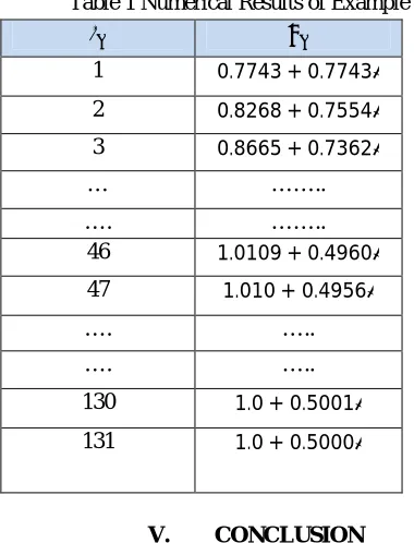
At 47 iteration ( ), p ( ) = p (1.010 + 0.4956i) = (0.0022 – 0.0176i):
The relative error in the real part at 47 iteration is 0.0869. The relative error in imaginary part at 47 iteration is 0.0579.
This solution at 47 iteration is close to the root calculated by Bairstow’s method i.e. (1 + 0:499i) At 131 iteration ( ), p( ) = p(1.0000+0.5000i) = (0.00011199-0.000013764i).
[image:4.612.193.383.435.684.2]The actual roots of ( ) are 0.5,−1.0, 2.0, (1 + 0.5 ) (1 – 0.5 ).
Table 1 Numerical Results of Example 1
1 0.7743 + 0.7743
2 0.8268 + 0.7554
3 0.8665 + 0.7362
… ……..
…. ……..
46 1.0109 + 0.4960
47 1.010 + 0.4956
…. …..
…. …..
130 1.0 + 0.5001
131 1.0 + 0.5000
V. CONCLUSION
iterative part directly with a single initial guess unlike the case of Bairstow’s method where number of pre-calculations are performed using recurrence relations using two initial guess as r and s.
VI. ACKNOWLEDGMENT
We thank the Department of Mechanical Engineering and Department of Production Engineering, Vishwakarma Institute of Technology, Pune for the guidance and support provided for carrying out this work.
REFERENCES [1]. J. Mathews, K. Fink, Numerical Methods Using MATLAB, Pearson Education., 2006.
[2]. D. Kincaid, W. Chency, “Numerical Analysis Mathematics of Scientific Computing,” Third edition. [3]. S. C. Chapra, R. Canale, “Numerical Methods of Engineers,” Mc Graw Hill Education., Seventh edition.