A Novel Blind Source Separation Approach Based on Invasive Weed Optimization

(1)

2018 International Conference on Communication, Network and Artificial Intelligence (CNAI 2018) ISBN: 978-1-60595-065-5

A Novel Blind Source Separation Approach Based on

Invasive Weed Optimization

Zhu-cheng LI

1,2

and Xiang-lin HUANG

1,*

1_{Faculty of Science and Technology, Communication University of China, Beijing 100024, China}

2_{Business College, Beijing Union University, Beijing 100025, China}

*Corresponding author

Keywords: BSS, IWO, Optimization algorithm, Negentropy.

Abstract. Traditional optimization algorithms for Blind Source Separation (BSS) are mainly based on the gradient, which requires the objective function to be continuous and differentiable, and have some defects such as slow convergence speed or poor accuracy of the solution. To solve these problems, a novel BSS approach based on Invasive Weed Optimization (IWO) is proposed in this paper. By maximizing a negentropy-based objective function, simulation experiments confirm the effectiveness of the proposed algorithm.

Introduction

Blind Source Separation [1,2] refers to the techniques which can estimate source signals using only several observed signals without prior knowledge of the source signals and mixing processing. “Cocktail Party Problem” is a vivid example for BSS problems: even in a noisy environment, you have ability to selectively attend to and recognize one source of auditory inputs. “Cocktail Party” scenario makes scholars more confident in solving the BSS problem. Jutten, Comon and Sorouchyari [3,4,5] published three classic articles focusing on blind signal separation, and these works made significant progress in the study of BSS problem. BSS algorithms often use a series of assumptions. The most common assumption is that source signals are statistically independent. The methods based on this assumption are called Independent Component Analysis (ICA) [1,6,7,8], which is statistical technique of decomposing several mixed signals into independent parts.

So far, BSS technologies have been widely used in many fields such as biomedical signal processing [9], image restoration and image encryption [10], sound recognition, antenna array processing, and mechanical faults diagnosis [11], and so on.

Conventional optimization algorithms for BSS are based on gradient. Unfortunately, the gradient technique requires the objective function to be continuous and differentiable, and is not suitable for locating the global optimum. In addition, the gradient methods can result in the conflict of convergence speed and accuracy. So, the use of the gradient is very limited.

The bio-inspired optimizations are inspired by the collective intelligence occurring through the natural biological evolution or the social behavior of such biological entities like a swarm of bees, a colony of ant, a flock of birds, a school of fish, and so on. The bio-inspired algorithms can be applied in a wide range, and do not require continuity and differentiability of the objective function. Compared with conventional gradient-based approaches, these techniques are characterized by higher accuracy, efficiency, and robustness, and have been gradually applied in BSS in the past few years, such as Genetic Algorithms (GA) [12], Particle Swarm Optimization (PSO) [12,13], and Artificial Bee Colony (ABC) [14], and so on.

(2)

In this paper, a new BSS algorithm based on IWO (IWO-BSS) is proposed. Simulation results prove the effectiveness of this method.

Blind Source Separation

Mathematical Model

This section lists the basic formulations of BSS and describes its key properties. Suppose some unknown source signals s

 

k _s k₁

   

,s₂ k , , s_n

 

k _T are input to an unknown linear system

whose input-output characterization is defined by nonsingular mixing matrix _{A R}_ m n ₍

mn).

With negligible noise, the m-dimensional vector of observation signals

 

1

   

, 2 , ,

 

T m k _x k x k  x k _

x is given by

 

k 

 

k

x As . (1)

The objective of BSS is to obtain the optimal separation matrix (de-mixing matrix)_W_n m

based only on the observed signals x such that

 

k 

 

k

y Wx . (2)

Here,

 

1

   

, 2 , ,

 

T n k _y k y k  y k _

y is the recovery signal vector. Ideally, the separation matrix W should be equal to_A1_{, so that}_{y s}_ _{. But}_y_{is only an estimate of}_s_{within the well-known} permutation and scaling ambiguities.

Objective Function- Negentropy

It can be known by the Central Limit Theorem that non-Gaussianity of any independent signal is stronger than one of their mixed signals, so non-Gaussianity can be used to measure whether mixed signals have been effectively separated. This is the essence of all ICA methods.

An important measure of non-Gaussianity is negentropy [6,7], which is based on differential entropy from the information-theoretic.

The entropy H of a discrete random variable yis classically defined as follows：

 



_i



log



_i



i

H y  



P ya P ya . (3)

Here, ai is the possible value of y, and P is the probability density function (PDF) ofy.

Correspondingly, the differential entropy H of a continuous-valued random vector y can be written

as

 

log

 

d

H y  



f y f y y. (4)

Here, f y

 

is the probability density function ofy. Negentropy J of yis defined as follows：

 



gauss



 

J y H y H y . (5)

Here, y_gauss is a Gaussian random variable of the same covariance matrix as y. Negentropy is

always nonnegative, and it is zero if and only if y follows Gaussian distribution. In fact, negentropy is a better measure means of non-Gaussianity than the conventional, cumulant-based one, as far as statistical property of each source signal can be accurately estimated.

(3)

 

2

 

2

 

4

 

2

   

3 4 3 3 4

1 1 7 1

12 48 48 8

i i i i i i

J y  k y  k y  k y  k y k y . (6)

Here, k_i denotes the ith-order cumulant of y. If the probability distribution of the signaly_i is

symmetric, thenk₃ 0, and

 

2

 

4 1 48

i i

J y  k y . (7)

Here, k4is called as kurtosis and can be defined as follows：

 

4 2 2

4 i i 3 i

k y E y _{ } E  _{ }y . (8)

The other approximation of negentropy based on the maximum entropy principle [6] is expressed as follows:

 



 











2

i i gauss

J y r E G y_ E G v _ . (9)

Here, r is a positive constant, G is a nonquadratic function, and v_gauss is a Gaussian variable with

zero mean and unit variance.

Invasive Weed Optimization

The basic IWO process [15] is refined as four sections imitating weed colonization: population initialization, growth and reproduction, spatial dispersal and competitive exclusion.

Population Initialization

A limited number of weeds are randomly dispread in an n-dimensional search (solution) space. The position of each weed is an initial solution for the optimization problem.

Growth and Reproduction

The weeds which have acquired more resources have a better chance of producing seeds, while those, which are less adapted to the field, reproduce less seeds. In other word, a plant will produce seeds based on its fitness, the colony’s lowest and highest fitness. This procedure can be illustrated by

 

min





max min min max min

i floor

f W f

NUM F S S S

f f



 

 _   _



 . (10)

Here, f_maxand f_min respectively represent the maximum and the minimum fitness value; F_floor

represents rounding down a function; S_maxand S_min represent the maximum and the minimum

number of the seeds respectively; f W

 

_i is the fitness value of the i-th weed.

Spatial Dispersal

The produced seeds in the previous time are distributed randomly in the space in the form of normal distribution with mean zero and a varying standard deviation_iter. By setting the mean equal to zero, the seeds are located randomly near to the parent plant. Decreasing the variance gradually, the fitter weeds are gathered together, and bad weeds are eliminated over time. The parameter_iter in every time may be described by



max







max n

iter n initial final final iter iter

iter

(4)

Here, itermaxand iterare respectively the maximum number of iteration cycles and the current iteration number; _initial and _final respectively represent the initial and final standard deviations; n

is the nonlinear modulation index.

Competitive Exclusion

When the population of weeds reaches its maximum, they are ranked together according to their fitness values. The weeds with the higher fitness are reserved, while the others are eliminated.

The above processes except population initialization continue until iteration reaches its maximum and hopefully the seed with best fitness is closest to the optimal solution.

A BSS Approach Based on IWO

The following is detail steps of BSS algorithm based on IWO (IWO-BSS).

•Step 1: Read the observed signalsx and center them to make their expectation zero, and then whitening the above output;

•Step 2: Produce a certain amount of separation matrixes as pioneer weeds; distribute them randomly in the search space;

•Step 3: Calculate the initial fitness value of each weed, and then rank them based on their fitness; •Step 4: Each weed produces a few new seeds using Eq. 10; the seeds are distributed randomly near the parent individuals based on Eq. 11;

•Step 5: These new seeds grow into new weeds and are ranked together with their parents according to their fitness. When the number of weeds in a colony reaches its maximum, the ones with lower ranking are eliminated, while the others are preserved;

•Step 6: If update number is less than maximum iteration, jump to Step 4; otherwise, output the optimal solution with best fitness in populations.

Simulation Experiments

To illustrate the performance of the proposed BSS algorithm, we compared it with BSS algorithm based on PSO (PSO-BSS).

Experimental Environment and Parameter Setting

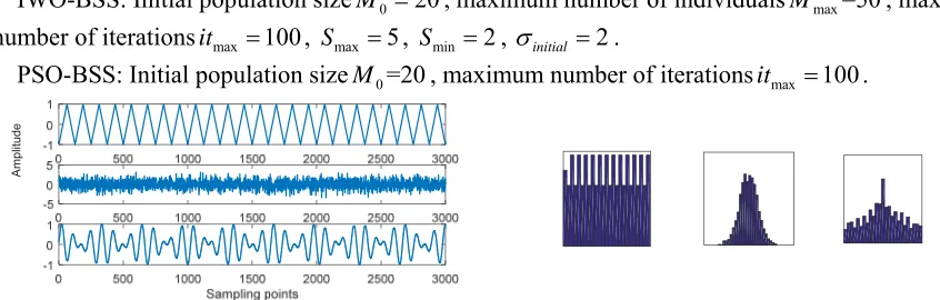
[image:4.612.83.506.547.682.2]

The left and right image of Fig. 1 respectively show three different source signals and their respective histograms. In the former, totally 3000 sampling points are set as abscissa and amplitude is set as ordinate. The mixed signals and their histograms are respectively shown in the left and right image of Fig. 2. The 3×3 mixing matrix A is random. The parameters of two algorithms are set as follows:

IWO-BSS: Initial population sizeM₀20, maximum number of individualsM_max=50, maximum

number of iterationsitmax 100, Smax 5, Smin 2, initial 2.

PSO-BSS: Initial population sizeM₀=20, maximum number of iterationsit_max 100.

A

m

p

litude

(5)

A

m

plitud

[image:5.612.89.506.66.281.2]

e

Figure 2. Mixed signals (Left) and their histograms (Right).

A

m

plitud

e

Figure 3. Restored signals (Left) and their histograms (Right).

The Results of Simulation and Analysis

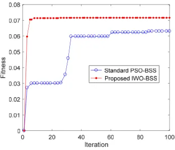
The left and right image of Fig. 3 is respectively the restored signals and their histograms obtained by IWO-BSS after 26 iterations. In contrast to Fig. 1 and Fig. 3, we can find that the new algorithm restores the source signals very well after 26 iterations. The mean fitness curves in Fig. 4 mean that IWO-BSS has the better behavior on accuracy and speed than PSO-BSS. Fig. 5 shows the scatter plots of three source signals versus three recovered signals by the proposed algorithm after 26 iterations. As can be seen from Fig. 5, the mixed signals are well restored, but most of their amplitudes and orders, comparing with those of the source signals, are be changed.

It is found from the data acquired from experiments that the performance of the new algorithm is superior to that of PSO-BSS: Firstly, after convergence, the fitness value of the proposed algorithm increases by 13 percent compared with that of PSO-BSS, from an average of 0.0631 to 0.0716; secondly, PSO-BSS needs approximately 87 iterations to converge, whereas IWO-BSS needs only 26 iterations.

[image:5.612.102.276.488.637.2]

Figure 4. Fitness curves obtained by different

optimization algorithms. Figure 5. Scatter plots of source signals versus restored signals.

Conclusion

[image:5.612.336.497.490.637.2]

(6)

and faster convergence speed. These features make the procedure suitable in many applications, even if their objective functions are discontinuous and nondifferentiable.

References

[1] X.C. Yu, H. Dan, J.D. Xu, Blind source separation: theory and applications, John Wiley & Sons, 2013.

[2] G.R. Naik and W. Wang, Blind source separation, Springer, Berlin, 2014.

[3] C. Jutten and J. Herault, Blind separation of sources, part I: An adaptive algorithm based on neuromimetic architecture, Signal processing, 24 (1991) 1-10.

[4] P. Comon, et al., Blind separation of sources, Part II: Problems statement, Signal processing, 24 (1991) 11-20.

[5] E. Sorouchyari, Blind separation of sources, Part III: Stability analysis, Signal processing, 24 (1991) 21-29.

[6] A. Hyvärinen and E. Oja, Independent component analysis: algorithms and applications, Neural networks, 13 (2000) 411-430.

[7] P. Comon, Independent component analysis, a new concept?, Signal processing, 36 (1994) 287-314.

[8] J.V. Stone, Independent Component Analysis, Wiley StatsRef: Statistics Reference Online, 2014. [9] M.S.H. Jadhav and M.D.N. Dhang, Extraction of Fetal ECG from Abdominal Recordings Combining BSS-ICA & WT Techniques, International Journal of Engineering, 10 (2017) 869-875. [10] N.A.M. Abbas, Image encryption based on independent component analysis and Arnold’s cat map, Egyptian Informatics Journal, 17 (2016) 139-146.

[11] M. Farhat, Y. Gritli, M. Benrejeb, Fast–ICA for Mechanical Fault Detection and Identification in Electromechanical Systems for Wind Turbine Applications, International Journal of Advanced Computer Science and Applications, 8 (2017) 431-439.

[12] S. Mavaddaty and A. Ebrahimzadeh, Blind signals separation with genetic algorithm and particle swarm optimization based on mutual information, Radioelectronics and Communications Systems, 54 (2011) 315-324.

[13] Q.Y. Li and H.Y. Quan, Analyze gravity tide signal based on ICA with PSO, 2015 IEEE International Conference on Signal Processing, Communications and Computing (ICSPCC), (2015) 1-4.

[14] Y. Xu, Y.F. Zhu, H.B. Shen, Blind source separation based on adaptive artificial bee colony algorithm, Transducer and Microsystem Technologies, 36 (2017) 127-130.