Balancing and Optimizing of Dispatching Schemes of Weekend Commuting Buses for Resident Students

2018 International Conference on Physics, Computing and Mathematical Modeling (PCMM 2018) ISBN: 978-1-60595-549-0

Balancing and Optimizing of Dispatching Schemes of Weekend

Commuting Buses for Resident Students

Han-pei LIU

, Xi-hui LIU

and Ai-min JI

Shenyang No.2 High School, China

2

Minnan Normal University, China

*

Corresponding author

Keywords: Dispatch of commuter buses, Massive transportation volume, Dijkstra algorithm, Non-linear planning model, Mileage balance.

Abstract. The dispatch of commuter buses with massive transportation volume is different from logistics transportation and distribution. It involves bus dispatch, region partition, path optimize, and travel distance balance etc. To tackle this problem, commuting region block planning is adopted to determine commuting stops, Dijkstra algorithm is used to determine the shortest travel route, the mileage balance constraint conditions is to construct non-linear planning model for peak covering problem, and Lingo system is used to solve it to get optimal travel path of commuter buses. The data demonstrates that the balanced and optimized school commuting dispatch plan can address the school commuting transportation problem.

Introduction

Transportation plays dominant role in industrial & agriculture production and daily life. The optimized dispatch of transportation has been studied by many researchers. For example, Wang et al. applied ant colony algorithm based data envelopment analysis (DEA) to simulation of rapid path planning problem for logistics transportation [1]. Jia et al. adopted grey correlation and improved Floyd algorithm to optimize cold-chain logistics dispatch path [2]; Wang used optimization method to tackle total transportation cost based garbage truck dispatch problem [3].

However, there are few reports on commuting dispatch problem in transportation. Moreover, massive transportation volume commuting is different from logistics transportation and distribution. On one aspect, passengers spread over a large area, and distribution sites and locations are stable. On the other aspect, as for massive transportation volume commute, many buses may pass passenger overridden area, so the buses may either stop for boarding or dropping people, or just bypass. Thus, the massive transportation volume dispatch problem involves bus dispatch, region partition, path optimize, and travel distance balance etc.

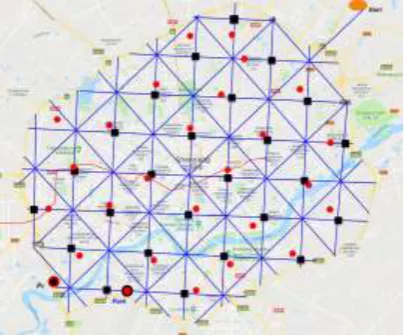
In a high school, senior 2 students come to school in new campus located in urban north. They reside in this campus from Monday to Thursday. At 16:30, Friday, transportation companies send commuters to take students to the commuter stations nearby their houses respectively, and then they come back home by themselves. On Sunday, the students need to board commuters at the commuter stations nearby their houses and return to the campus. There are 426 students spreading over the third ring road area enclosed by G1 and G1501 beltways as shown in Fig. 1. This paper studied the above dispatch problem. To ensure that the students that can arrive at home before 6 PM, a method was presented to plan reasonable transportation plans and achieve minimum transportation cost.

The Determination of Commuting Stations’ Locations

inside the square to the center is always less than 3.5 2 / 22.5kilometers. Take the walking speed as 5 kilometers per hour, then every student can arrive at home in 30 minutes.

However, this kind of deployment is inevitable to misplace commuter stations. The stations may appear in no-parking road sections, one-way street or even roadless places. Hence, it’s necessary to move these stations to main roads, crossroads or near the underground, as little spots shown in Fig. 1. This ensures the safety of students, and the commuter buses will not block the roads in the peak-hour of commuting. 25 commuting stations are obtained, which are denoted by capital letters with brackets: A(9) ,B(9) ,C(7) ,D(6)……Y(12) ,Z(15). The letters depict the serial number of the stations, and the digits in the brackets depicts the number of commuting students using the corresponding station. For convenience, let S depict the start point and get S(426) (426 is the total commuting students). Meanwhile, the car park is incorporated to the nearby commuter station and get P(13). This reduces the computation and speed up the algorithms for path optimization.

Figure 1. Distribution of resident students and locations of commuting stations.

Driving Direction and Distance between Stations

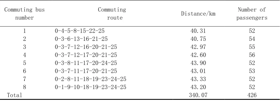
The path corresponding to the minimum driving time between adjacent stations can be obtained by Google GPS navigation system and Dijkstra algorithm in toolbox of MATLAB. As figure 2 shows, a commuting station of the road network is depicted as a node of the graph, and the road linking two stations is depicted as an edge linking the corresponding nodes. The length or the road is depicted as the weight of the edge. Thus, the road network is expressed as the weighted network graph. In Fig. 2, the network linked by the solid edges represents actual driving routes of the commuters. The directed network linked by imaginary lines represents the directions, routes and minimum distance of commuting buses between the adjacent stations. It needs to discard the congested roads in peak hour (e.g. route I-K and K-Q paths) and retrograde (the direction pointing to S point) ways (e.g. A-B, C-D, E-F, G-F, H-G, I-H, F-N, O-L, J-K and T-R paths). Once these paths are deleted, the directed imaginary edges between the adjacent stations represent the feasible paths and directions which the commuter buses can choose. The number of imaginary lines refer to minimum distances between stations. Take B-H adjacent stations as an example, the commuters can only drive from station B to station H, and the minimum distance is 3.13 kilometers. Thus, a 2626 adjacency matrix W is constructed. If there are roads between the stations, the corresponding weight is greater than 0. If there are no roads between the stations, the corresponding weight is set as infinite. Use the sparse (W)

command in MATLAB to gain sparse matrix w of the adjacent matrix W.

The Balance and Optimization of Transporting Schemes

passengers and transportation company are consistent with the optimal evaluation index, i.e. the shortest commuting time. Passengers hope to come back home as fast as possible. The transportation company also expect to finish the commuting task as soon as possible to undertake more transportation tasks.

Consequently, the problem can be described as: given the initial and final positions of commuting, the number and position of passengers, the constraints of allowed passenger capacity and transport mileage, determine proper number of commuting buses and reasonable transport routes to achieve the shortest commuting time.

Based on the above description of this problem, the facts and assumptions can be derived as following:

1) There are one start point, one end point (parking area) and 25 stops. The number of passengers of each stop is definite.

2) Each commuting bus has weight capacity limit and they are of same models. 3) Same traffic condition for every car with an average speed of v.

4) Do not consider the effect of traffic lights when the bus drives between the stops. 5) The time is same for the buses to stay at each stop, let it be 6 minutes average, i.e. 0.1h.

Figure 2. Driving directions, routes and distances between adjacent stations.

Building the Model

Assume the number of commuting stations is n (where n=26, including start point S), numbered from

0 to 25, and each commuter station is considered as a vertex of a directed graph, denoted by Vi (i=0, 1, … n). The value of Vi is the number of students at the commuting station, and the shortest path between two stations is denoted by wij (i=0, 1, … n; j=1, 2, … n). The allowed maximum number of passengers is denoted by q. The number of buses required is denoted by m. To establish the model, we also need to define the following decision variables:

,

1 Buses driving form stop to , 0,1, 2,... , 1, 2 , 1 2...

0 Otherwise

i j

ij k

V V i n j n k m

r      



，

(1)

,

1 Stop ' commmuting tasks performed by bus , 1, 2,... ; 1, 2...

0 Otherwise

i i k

V s k i n k m

e    

 ₍₂₎

The objective function of the mathematical model is:

, , ,

1 0 0 1 1

min ( ) /

m n n m n

ij k ij k i k

k i j k i

t w r v T e

    







, 1 , 1 , , 0 , , 1 , 0 , 1

1 2 1, 2,...,

1, 2,...

1, 2,... ; 1, 2,...

. .

0,1,... ; 1, 2,...

1 j 1, 2,... ; 1, 2,...

m i k k n i k i n

ij k i k i

n

ij k i k j n ij k i n ij k j

e k m

V q k m

r e j n k m

s t

r e i n k m

r n k m

r                    











1 i 0,1,... ;n k 1, 2,...m                  _{  }





In the practical situation of commuting process, different buses have different mileages because of

different driving routes and stops. To narrow the difference, the distance balance () is defined as

follow: max min 1 ( ) ( ) / m k k d d d m    



, 1,2,... 0 1

n n

k ij ij k k m

i j

d w r _

 





max max{ ,1 2,... m}

d  d d d Denotes the maximum driving distance of No. k bus;

min min{ ,1 2,... m}

d  d d d Denotes the minimum driving distance of No. k bus.

Therefore, commuting problems also need to add another objective optimization function, which is, minimizing the equilibrium of driving distance.

max min

, 1 0 1

( )

min =

( ) /

m n n

ij ij k k i j

d d

w r m 

  





(6) Consequently, the commuting problem becomes a multi-objective optimization problem with two objective functions.

The Solution of Multi-objective Optimization

Multi-objective problem solving is more complex. The actual solution process turns the multi-objective problem into a single objective optimization problem. Considering the correlation between the minimum time objective optimization function and the balance degree, the minimum balance degree objective function is transformed into a constraint   ₀, where ₀ is an allowable

deviation value. Take the road condition and traffic lights into account, and let ₀ 10%, then we

can get:

max min

, 1 0 1

( )

= 10%

( ) /

m n n

ij ij k k i j

d d

w r m 

  

 _



Take the passenger capacity of commuting bus q=56 and the total number of commuting students Q=426 into the following formula:

INT( / )+1

m Q q ₍₈₎

where, INT() in eq.(8) is a rounding function, then solve that the number of commuting bus m=8.

Set V { , ,...V V_{0 1} V₂₅} as vertices, E as the edge between the vertices and W as the adjacency matrix to construct the weight graph G( , ,V E W), then the model of commuting problems, for instance, eq. (1)~(3), eq. (6) can be viewed as a nonlinear programming model of vertex coverage problem, and Lingo software can be used to develop a program for a solution.

Take v=60km/h, m=8, the sparse matrix w and the data in Table 1 into the developed Lingo program and obtain the results as shown in Table 2.

Table 1. Commuting station information.

Commutin g stations

number 0 1 2 3 4 5 6 7 8 9 1 0 1 1 1 2 1 3 1 4 1 5 1 6 1 7 1 8 1 9 2 0 2 1 2 2 2 3 2 4 2 5 Commutin g stations

location S A B C D E F G H I J K L M N O Q R T U V W X Y Z P Commutin

g students

number 0 9 9 7 6 7 8 2 6 2 5 1 1 2 2 2 7 2 9 2 2 8

1 1 3 3 2 7 2 0 1 8 2 2 2 4 1 5 1 5 1 2 1 3

Table 2. Optimization algorithm to solve the results.

Commuting bus number

Commuting

route Distance/km

Number of passengers

1 0-4-5-8-15-22-25 40.31 52 2 0-3-6-13-16-21-25 40.75 54 3 0-3-7-12-16-20-21-25 42.97 55 4 0-3-7-12-17-20-21-25 42.60 56 5 0-3-8-11-17-20-24-25 43.90 52 6 0-3-7-11-17-20-21-25 43.01 53 7 0-2-8-11-18-19-23-24-25 43.33 52 8 0-1-9-10-18-19-23-24-25 43.20 52

Total 340.07 426

Data Analyzing

Analyzing the data of mileage in Table 2, we can obtain that the balance degree of 8 commuting buses’ driving distances is 8.45%. Obviously, it meets that the balance degree is less than 10% specified in eq. (7).

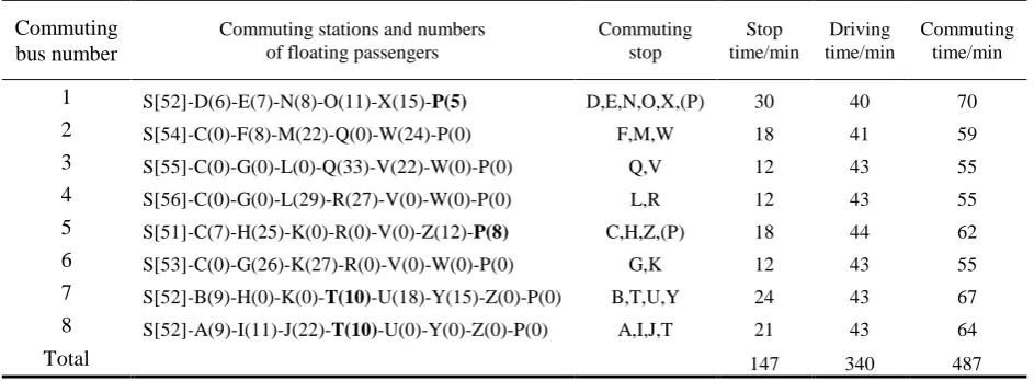
The commuting path obtained by the optimization algorithm is transformed into corresponding commuting stops and passengers. The driving time is calculated according to the stopping time. Then the driving routes and analysis of 8 commuting buses are obtained and shown in Table 3. It can be seen from the Table 3, both No.1 and No.5 commuting bus stop at the station P for the passengers. Moreover, both No.7 and No.8 commuting bus also stop at the station T. Two commuting buses accomplish the commuting mission at the same station together, which is the complexity of commuting problem more than ordinary transportation and distribution.

passengers require at most 70+18.68=88.68min from P0 to get home. Hence, if the commuting buses

depart at 16:30 punctually from the initial station, the passengers whose home is farthest can arrive home before 18:00.

Conclusion

This paper studied the commuting buses dispatch problem for a high school. The commuting area is divided into 25 commuting stations, and it concludes that 5 buses with 53 seats and 3 buses with 56 seats are required for the commuting. We build a nonlinear programming model of vertex coverage problem and develop Lingo program to gain access to a solution. Finally, it computes the driving routes of 8 buses, and the mileage of each bus is between 40 and 44km with distance balance of 8.45%. The solved dispatch solution is optimal in buses arrangement, area partition, commuting routes, time and the balance. This solution can ensure that all passengers arrive home on the schedule. The commuting is efficient and effective, and the commuting cost can be reduced to the least.

Table 3. Results analyzing.

Commuting bus number

Commuting stations and numbers of floating passengers

Commuting stop

Stop time/min

Driving time/min

Commuting time/min

1 _{S[52]-D(6)-E(7)-N(8)-O(11)-X(15)-P(5) D,E,N,O,X,(P) 30 40 70}

2 S[54]-C(0)-F(8)-M(22)-Q(0)-W(24)-P(0) F,M,W 18 41 59

3 _{S[55]-C(0)-G(0)-L(0)-Q(33)-V(22)-W(0)-P(0) Q,V 12 43 55}

4 _{S[56]-C(0)-G(0)-L(29)-R(27)-V(0)-W(0)-P(0) L,R 12 43 55}

5 S[51]-C(7)-H(25)-K(0)-R(0)-V(0)-Z(12)-P(8) C,H,Z,(P) 18 44 62

6 _{S[53]-C(0)-G(26)-K(27)-R(0)-V(0)-W(0)-P(0) G,K 12 43 55}

7 _{S[52]-B(9)-H(0)-K(0)-T(10)-U(18)-Y(15)-Z(0)-P(0) B,T,U,Y 24 43 67}

8 S[52]-A(9)-I(11)-J(22)-T(10)-U(0)-Y(0)-Z(0)-P(0) A,I,J,T 21 43 64

Total _{147 340 487}

Note: [] is the number of passengers boarding, () is the number of passengers getting off.

References

[1]Ning-Zhong Shi. Training and Teaching of Subject Core—Take math as an example[J], Rimary

and Secondary School Management, 2017(01):36-37.

[2]Cai-Yan Zhang. Analysis of core in mathematics: Connotation, Value and Training Road[J],

Educational Journal, 2017(01):60-64.

[3]You-Jun Liu. Research The Implement core literacy in Mathematics Class[J], Chinese off

Campus Education, 2016(10):57-58.

[4]Li-Feng Wang, Shuang-Shuang Liu. Logistics Transportation Rapid Distribution Path Planning