2019 International Conference on Computation and Information Sciences (ICCIS 2019) ISBN: 978-1-60595-644-2
A Priori Indicator of Convergence Rate for
Power Method for Computing the Spectral
Radius of Saddle Point Matrices
Zheng Li, Tie Zhang and Changjun Li
ABSTRACT
Saddle point matrix is the coefficient matrix of the linear system derived from the saddle point problem, which arise from many scientific and engineering applications. The eigenvalue information of the saddle point matrices is usually quite important in practical computation. In this paper, the power method is applied to computing the spectral radius of the saddle point matrices. Furthermore, based on some theoretical results of eigenvalue estimates for the saddle point matrices, a new indicator, which is a function of the extreme eigenvalues of the sub blocks, is proposed to predict the convergence rate of the power method. The numerical results of the experiment on computing the spectral radius of the saddle point matrices derived from the model of the Stokes equation demonstrate that the proposed algorithm and the indicator are both effective.
1. INTRODUCTION
Saddle point problems arise from many scientific research fields and engineering applications, such as mixed finite element methods, constrained least square problems, image processing and so on [1-16], and usually generate the following linear system:
( 𝑨 𝑩 𝑩T 𝑶) (
𝒙
𝒚) = (𝒃𝒒). (1)
This system is also called “augmented system” [1, 4] or “KKT system” [1], and its coefficient matrix
𝑾 = ( 𝑨𝑩T 𝑩𝑶) (2) is called “saddle point matrix” [10-16]. Here the sub block 𝑨 ∈ R𝑚×𝑚 is symmetric and positive definite, 𝑩 ∈ R𝑚×𝑛 (𝑚 ≥ 𝑛) has full column rank, and 𝑶 is an n-order
Zheng Li, Department of Mathematics, Northeastern University, Shenyang, 110004, P.R. China
Tie Zhang, Department of Mathematics, Northeastern University, Shenyang, 110004, P.R. China
zero matrix. Matrix 𝑾 is symmetric and indefinite [1], and has a peculiar block structure. In order to make better use of the sparsity of 𝑾 in large-scale computation, researchers have developed various efficient algorithms over the past 30 years [1-8]. As far as we know, the focus of current research has shifted to the preconditioning techniques for accelerating the convergence rate of the iteration algorithms. Most of these techniques need eigenvalue information of matrix 𝑾 (or other related matrices). Therefore, the research on the properties of the key eigenvalues of saddle point matrix has attracted more attentions [9-16]. We should note that in practice the size of matrices are usually very large, and the computational complexity should be as small as possible. On the other hand, sometimes the eigenvalues of sub blocks 𝑨 and
𝑩 may be obtained in advance by some simple methods. The inexpensive information should be fully utilized.
In this paper, we introduce the power method to compute the spectral radius, i.e., the maximum eigenvalue modulus of the saddle point matrix 𝑾, and establish a concrete program according to the specific structure of 𝑾. Furthermore, based on the theoretical results of some classical references we propose a new priori indicator, which depends on the maximum and minimum eigenvalues (or singular values) of sub blocks 𝑨 and 𝑩, to predict the convergence rate of power method. In the experiment, we test this method with P1-P0 mixed finite element model. Numerical results demonstrate that the involved algorithm and indicator are both valid.
We use following notations throughout this article. The eigenvalues of saddle point matrix 𝑾 are denoted in descending order as: 𝜆1 ≥ 𝜆2 ≥ ⋯ ≥ 𝜆𝑚+𝑛. The
symbols |𝜆̃1| and |𝜆̃2| represent the largest and the second largest eigenvalue
modulus of 𝑾 respectively. The eigenvalues of the sub block 𝑨 are denoted by
𝜇1 ≥ 𝜇2 ≥ ⋯ ≥ 𝜇𝑚 (> 0), and the singular values of sub block 𝑩 are denoted by
𝜎1 ≥ 𝜎2 ≥ ⋯ ≥ 𝜎𝑛 (> 0). In this article we assume the eigenvalues of 𝑨 and singular values of 𝑩 are easily obtained in advance. The notation |∙| represents the modulus (absolute value) function of the real number. The sign 𝜆𝑘(∙) denotes the k-th
largest eigenvalue of the involved (symmetric) matrix. In addition, the notation “𝑿 ≼ 𝒀” means 𝒀 − 𝑿 is symmetric and semi positive definite.
2. MAIN RESULTS
2.1 Basic Theory on the Eigenvalues of Saddle Point Matrix
We start the discussion with a brief review of some basic theory. First of all, let us recall some classical useful theoretical results for the general symmetric matrices.
Lemma 1 (Corollary of Weyl Theorem) [17] If 𝑿 and 𝒀 are both symmetric matrices, and 𝑿 ≼ 𝒀, then 𝜆𝑘(𝑿) ≤ 𝜆𝑘(𝒀).
Lemma 2 (Sturm) [17] Assume 𝑾̃ ∈ 𝑅𝑀×𝑀 is symmetric, and 𝑨̃𝑚 is an arbitrary m-order principle sub matrix of 𝑾̃, then it holds that
𝜆𝑀−𝑚+𝑘(𝑾̃) ≤ 𝜆𝑘(𝑨̃ ) ≤ 𝜆𝑚 𝑘(𝑾̃), 1 ≤ 𝑘 ≤ 𝑚 ≤ 𝑀.
Moreover, for the eigenvalue distribution of saddle point matrix, there is a particularly important result as follows.
Lemma 3 (Rusten)[1, 2] Let saddle point matrix 𝑾 and its sub blocks 𝑨 and 𝑩
𝛬(𝑾) ⊆ 𝐼 = 𝐼−⋃𝐼+, where
𝐼− = [1
2(𝜇𝑚− √𝜇𝑚2 + 4𝜎1 2) , 1
2(𝜇1− √𝜇1 2+ 4𝜎
𝑛2) ], and
𝐼+ = [𝜇
𝑚, 12(𝜇1+ √𝜇12+ 4𝜎12)]. (3)
Remark: Lemma 2 and Lemma 3 indicate that the eigenvalues of 𝑾 and 𝑨 satisfy the following relation:
1
2(𝜇1+ √𝜇12+ 4𝜎12) ≥ 𝜆1 ≥ 𝜇1 ≥ 𝜆2 ≥ 𝜇2… ≥ 𝜆𝑚 ≥ 𝜇𝑚 > 0
> 12(𝜇1− √𝜇12+ 4𝜎
𝑛2) ≥ 𝜆𝑚+1≥ ⋯ ≥ 𝜆𝑚+𝑛≥ 12(𝜇𝑚− √𝜇𝑚2 + 4𝜎12). (3)
2.2 Power Method for Saddle Point Matrix
Power method has a simple scheme and is suitable to compute the largest eigenvalue modulus of the symmetric matrix [18, 19]. According to the structure of saddle point matrix 𝑾, we establish a program of power method [18] as follows.
Algorithm 1. Power Method for Saddle Point Matrix 1. Input the sub blocks 𝑨, 𝑩 of matrix 𝑾, start with vector 𝒙 = 𝒙0∈ R𝑚 and 𝒚 = 𝒚0∈ R𝑛; set
threshold 𝜀 for the stop criterion 2. For k=1, 2,…
3. 𝒖 = 𝒙/√𝒙T𝒙 + 𝒚T𝒚, 𝒗 = 𝒚/√𝒙T𝒙 + 𝒚T𝒚 4. 𝒙 = 𝑨𝒖 + 𝑩𝒗, 𝒚 = 𝑩T𝒖
5. 𝜃 = 𝒖T𝒙 + 𝒗T𝒚
6. If √(𝒙 − 𝜃𝒖)T(𝒙 − 𝜃𝒖) + (𝒚 − 𝜃𝒗)T(𝒚 − 𝜃𝒗) < 𝜀|𝜃| , Stop 7. End for
8. Accept 𝜌̂ = 𝜃 as the approximate value of the largest eigenvaue by modulus of 𝑾
Some upper bound of the convergence rate of the power method is characterized by the ratio |𝜆̃2| |𝜆̃⁄ 1| [19]. Generally speaking, the smaller the ratio |𝜆̃2| |𝜆̃⁄ 1| is, the faster the algorithm converges. Unfortunately, the ratio |𝜆̃2| |𝜆̃⁄ 1| is usually unknown before computation, thus we cannot set it as a priori indicator. Our desire is finding a practical priori indicator to predict the convergence rate of the power method.
2.3 A New Indicator of Convergence Rate
Rusten [2] has pointed out that some bounds of Lemma 3 are sharp, that is,
𝜆1 ≈12(𝜇1+ √𝜇12+ 4𝜎12), 𝜆𝑚+𝑛 ≈12(𝜇𝑚− √𝜇𝑚2 + 4𝜎12). (4)
A large number of numerical results (of this article, including reported and unreported numerical results) support this view. Based on condition (4) we propose following result.
Proposition 1 Under the assumption of (4), the largest eigenvalue modulus of saddle point matrix 𝑾 is |𝜆1|, and the second largest eigenvalue modulus should be
𝑚𝑎𝑥{|𝜆2|, |𝜆𝑚+𝑛|}.
|𝜆1| − |𝜆𝑚+𝑛| ≈ |12(𝜇1+ √𝜇12+ 4𝜎12)| − |12(𝜇𝑚− √𝜇𝑚2 + 4𝜎12)|
=12(𝜇1+ √𝜇12+ 4𝜎
12) −12(√𝜇𝑚2 + 4𝜎12− 𝜇𝑚)
=12(𝜇1+ 𝜇𝑚) +12(√𝜇12+ 4𝜎12− √𝜇𝑚2 + 4𝜎12) > 0. (5)
which means 𝜆1 has the largest modulus among all the eigenvalues of 𝑾, and then
the second largest eigenvalue modulus should be the maximum of |𝜆2| and |𝜆𝑚+𝑛|.
The proof is completed.
It follows from Proposition 1 and (4) that
|𝜆𝑚+𝑛|
|𝜆1| ≈ 1
2(√𝜇𝑚2+4𝜎12−𝜇𝑚) 1
2(𝜇1+√𝜇12+4𝜎12)
= √𝜇𝑚
2+4𝜎 12−𝜇𝑚
𝜇1+√𝜇12+4𝜎12
. (5)
In addition, (3) shows that 𝜆2 ∈ [𝜇2, 𝜇1]. We use the midpoint of interval [𝜇2, 𝜇1] as a probabilistic approximation of the value of 𝜆2, i.e., 𝜆2 ≈12(𝜇1+ 𝜇2). Therefore,
|𝜆2|
|𝜆1|≈ 1 2(𝜇1+𝜇2) 1
2(𝜇1+√𝜇12+4𝜎12)
= 𝜇1+𝜇2
𝜇1+√𝜇12+4𝜎12
. (6)
According to (5) and (6), now we propose the following indicator:
𝜒 = max {√𝜇𝑚
2+4σ 1 2−𝜇
𝑚
𝜇1+√𝜇12+4σ12
, 𝜇1+𝜇2
𝜇1+√𝜇12+4𝜎12
}. (7)
which is expected to be an effective approximation of the ratio |𝜆̃2|/|𝜆̃1| since
𝜒 ≈max{|𝜆𝑚+𝑛|, |𝜆2|}
|𝜆1| . The advantage of this new indicator is that it only relies on
some eigenvalues or singular values of sub blocks 𝑨 and 𝑩, and avoids the computation for the eigenvalues of 𝑾.
3. NUMERICAL EXPERIMENT
Following stationary Stokes equation is a classical problem in computational fluid dynamics [1, 3, 20]:
{
−𝜏Δ𝒖 + ∇𝑝 = 𝒇, in Ω; div 𝒖 = 0, in Ω;
∫ 𝑝dΩ = 0;
Ω
𝒖|∂Ω = 𝐠,
where Ω = (0,1) × (0,1) is a unit square domain, and ∂Ω is the boundary of Ω. Vector u represents the velocity, and p stands for the pressure. The constant 𝜏 > 0 is the viscosity coefficient [1]. We take P1-P0 mixed finite element method on the mixed triangular grids to discrete the stationary Stokes equation and derive the saddle point system as (1) (see [20] for details), which has the coefficient matrix as (2).
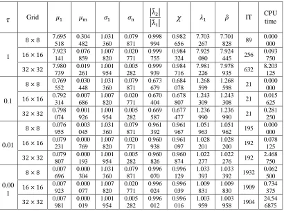
threshold 𝜀 = 0.001. The maximum and minimum eigenvalues of 𝑨, the maximum and minimum singular values of 𝑩, the values of ratio |𝜆̃2| |𝜆̃⁄ 1|, the values of indicator 𝜒, the maximum eigenvalue of 𝑾, the computed spectral radius 𝜌̂, the iteration times (IT) and the CPU time cost in each case are all reported in Table 1.
Some interesting phenomena emerged. In comparison, the algorithm converges fastest when 𝜏 = 0.1, and slowest when 𝜏 = 0.001. The values of the ratio
|λ̃2| |⁄ λ̃1| and the indicator 𝜒 are very close in each case, and in most case they are
monotonically related to the convergence rates. A seemingly "anomalous" phenomenon is that the performance of the ratio |λ̃2| |⁄λ̃1| (and the indicator 𝜒) is
not consistent with the convergence rate in case 𝜏 = 1. We think the reason is that the ratio |λ̃2| |⁄ λ̃1| only determines some upper bound of the convergence rate, so it is possible that the ratio |λ̃2| |⁄ λ̃1| has a large value but the convergence rate is still
[image:5.612.97.507.334.638.2]fast. In conclusion, numerical results show that Algorithm 1 is competent for the computation of spectral radius of saddle point matrix, and indicator χ is an effective substitute for the ratio |λ̃2| |⁄ λ̃1|.
TABLE I. NUMERICAL RESULTS OF ALGORITHM 1 ON STOKES EQUATION.
𝜏 Grid 𝜇1 𝜇m 𝜎1 𝜎n |λ̃2|
|λ̃1| 𝜒
𝜆1 𝜌̂ IT CPU time
1
8 × 8 7.695
518 0.304 482 1.031 360 0.079 871 0.998 994 0.982 656 7.703 267 7.701
828 89
0.000 000
16 × 16 7.923
141 0.076 859 1.007 820 0.020 771 0.999 755 0.984 324 7.925 080 7.924
445 256
0.093 750
32 × 32 7.980
739 0.019 261 1.001 954 0.005 282 0.999 939 0.984 716 7.981 226 7.978
935 632
8.203 125
0.1
8 × 8 0.769
552 0.030 448 1.031 360 0.079 871 0.673 679 0.684 078 1.268 599 1.268
598 21
0.000 000
16 × 16 0.792
314 0.007 686 1.007 820 0.020 771 0.670 404 0.678 807 1.243 309 1.243
308 21
0.015 625
32 × 32 0.798
074 0.001 926 1.001 954 0.005 282 0.669 587 0.677 477 1.236 990 1.236
990 21
0.281 250
0.01
8 × 8 0.076
955 0.003 045 1.031 360 0.079 871 0.961 392 0.961 967 1.051 963 1.051
962 195
0.000 000
16 × 16 0.079
231 0.000 769 1.007 820 0.020 771 0.960 938 0.961 097 1.028 201 1.028
200 192
0.078 125
32 × 32 0.079
807 0.000 193 1.001 954 0.005 282 0.960 826 0.960 874 1.022 277 1.022
276 192
2.468 750
0.00 1
8 × 8 0.007
696 0.000 304 1.031 360 0.079 871 0.996 070 0.996 129 1.033 393 1.033 392 1932
0.062 500
16 × 16 0.007
923 0.000 077 1.007 820 0.020 771 0.996 024 0.996 039 1.009 831 1.009 830 1909
0.734 375
32 × 32 0.007
981 0.000 019 1.001 954 0.005 282 0.996 012 0.996 016 1.003 959 1.003 958 1904
4. CONCLUSIONS
In this paper, we apply power method to computing the spectral radius of the saddle point matrices, and propose an effective priori indicator to predict the convergence rate. The present numerical results are in line with our expectations. However, we have to note that the discussion in this article relies on some approximate calculation. Further rigorous theoretical analysis and more numerical experiments are needed to verify the reliability of the new proposition.
ACKNOWLEDGEMENTS
This work was supported by the National Natural Science Funds of China (No. 11371081) and the State Key Laboratory of Synthetical Automation for Process Industries Fundamental Research Funds, China (No. 2013ZCX02).
REFERENCES
1. Benzi, M., G.H. Golub and J. Lieson. 2005. “Numerical solution of saddle point problems,” Acta. Numer., 14: 1-137.
2. Rusten, T. and R. Winther. 1992. “Preconditioned iterative method for saddle point problems,” SIAM J. Matrix Anal. Appl., 13(3): 887-904.
3. Elman, H.C. and D.J. Silvester. 1996. “Fast nonsymmetric iteration and preconditioning for Navier–Stokes equations,” SIAM J. Sci. Comput., 17(1): 33-46.
4. Fischer, B., A. Ramage, D.J. Silvester and A.J. Wathen. 1998. “Minimum residual methods for augmented systems,” BIT, 38(3): 527-543.
5. Bai, Z.-Z., G.H. Golub and M.K. Ng. 2003. “Hermitian and skew-Hermitian splitting methods for non-Hermitian positive definite linear systems,” SIAM J. Matrix Anal. Appl., 24(3): 603-626. 6. Bai, Z.-Z. 2009. “Optimal parameters in the HSS-like methods for saddle point problems,” Numer.
Linear Algebra Appl., 16(6): 447-479.
7. Li, C.-J., Z. Li, X.-H. Shao, Y.-Y. Nie and D.J. Evans. 2004. “Optimum parameter for the SOR-like method for augmented systems,” Int. J. Comput. Math., 81(6): 749-763.
8. Li, Z., C.-J. Li, D.J. Evans and T. Zhang. 2005. “Two-parameter-GSOR method for the augmented system,” Int. J. Comput. Math., 82(8): 1033-1042.
9. Simoncini, V. and M. Benzi. 2004. “The spectral properties of the Hermitian and skew-Hermitian splitting preconditioner for saddle point problems,” SIAM J. Matrix Anal. Appl., 26(2): 377–389. 10. Axelsson, O. and M. Neytcheva. 2006. “Eigenvalue estimates for preconditioned saddle point
matrices,” Numer. Linear Algebra Appl., 13(4): 339-360.
11. Huang, T.-Z., S.-L. Wu and C.-X. Li. 2009. “The spectral properties of the Hermitian and skew-Hermitian splitting preconditioner for generalized saddle point problems,” J. Comput. Appl. Math., 229(1): 37-46.
12. Shen, S.-Q., T.-Z. Huang and J. Yu. 2010. “Eigenvalue estimates for preconditioned nonsymmetric saddle point matrices,” SIAM J. Matrix Anal. Appl., 31(5): 2453-2476.
13. Shen, S.-Q., L. Jian, W.-D. Bao and T.-Z. Huang. 2014. “On the eigenvalue distribution of preconditioned nonsymmetric saddle point matrices,” Numer. Linear Algebra Appl., 21(4): 557-568.
14. Li, Z., T. Zhang and C.-J. Li. 2009. “An improved interval estimate for the maximum eigenvalues of saddle point matrices,” J. Northeast. Univ. Nat. Sci., 30(9): 1362-1364.
15. Ruiz, D., A. Sartenaer and C. Tannier. 2018. “Refining the lower bound on the positive eigenvalues of saddle point matrices with insights on the interactions between the blocks,” SIAM J. Matrix Anal. Appl., 39(2): 712-736.
17. Wang, S.-G., M.-X. Wu and Z. Z. Jia. 2006. “Matrix Inequalities,” Bejing, Science Press.
18. Bai, Z.-J., J. Demmel, J. Dongarra, A. Ruhe and H. van der Vorst. 2011. “Templates for the Solution of Algebraic Eigenvalue Problems A Practical Guide,” Beijing, Tsinghua University Press. 19. Golub, G.H. and C.F. Van Loan. 2014. “Matrix Computations (4th Edition),” Beijing, Posts &
Telecom Press.