RESEARCH ARTICLE
Virtual-dynamics-based reference gait
speed generator for limit-cycle-based bipedal
gait
Taisuke Kobayashi
1*, Kosuke Sekiyama
2, Yasuhisa Hasegawa
2, Tadayoshi Aoyama
2and Toshio Fukuda
3,4Abstract
This paper addresses a reference gait speed generator for limit-cycle-based bipedal gait of humanoid robots in order to achieve secure and efficient acceleration and deceleration without falling down at respective gait speeds. The ref-erence gait speed generator is hard to be developed by analytical approaches due to the necessity of barren work for identifying the respective basins of attraction. We challenge this issue by designing virtual dynamics among a robot, a virtual leader point, and a goal, and adapting it according to a falling risk of the robot. The virtual dynamics, which has settling and acceleration times as design parameters, gives the reference speeds derived from states of the robot and the leader point to a gait speeds controller. In the dynamics, the robot’s mass is optimized virtually to maximize efficiency while ensuring stability stochastically by using a selection algorithm for locomotion. Even when there were obstacles or an up slope in traveling courses of simulations, the robot achieved the autonomous traveling from the start to the goal securely. Specific resistance was also kept small in comparison with local-stability-based walking. The proposed method makes the limit-cycle-based bipedal gait more practical and contributes toward replacing the major method that ensures stability of every step.
Keywords: 3-D bipedal gait, Artificial potential field, Leader-follower control, Stochastic optimization
© The Author(s) 2018. This article is distributed under the terms of the Creative Commons Attribution 4.0 International License (http://creat iveco mmons .org/licen ses/by/4.0/), which permits unrestricted use, distribution, and reproduction in any medium, provided you give appropriate credit to the original author(s) and the source, provide a link to the Creative Commons license, and indicate if changes were made.
Introduction
In the research fields of humanoid robots, bipedal gait control to travel in a variety of environments, such as disaster sites, human-living buildings, etc., is an essen-tial issue. Limit-cycle-based bipedal gait [1–7] has excellent mobility in terms of energy efficiency from utili-zation of natural dynamics of robots, in contrast to major approach, which wastes the energy to ensure the stability of every step [8, 9]. This approach, however, makes foot-step planning (i.e., the robot’s global position control) more challenging compared to the major approach to ensure the stability of every step [10, 11], although a few studies achieved footstep planning by combining several stable gait primitives [7].
Such energy-efficient but less-controllable gait is there-fore suitable for traveling on large and long spaces where the footstep planning is not required. Instead of the foot-step planning, gait speed control is easily achieved in the limit-cycle-based bipedal gait. Gait speed controllers consist of three types: forward speed control [2–4]; side-ward speed control [3, 4]; and turning speed control [5, 6,
12]. Our approach, namely quasi-passive dynamic auton-omous control (Q-PDAC) with adaptive speed controller (ASC) [4, 5], has achieved all types of speed control. In addition, an autonomous transition between walking and running has been implemented to expand capabilities of the bipedal gait [13].
Q-PDAC with ASC has solved the gait speed con-trol adaptively, not analytically. This concept may cause falling down when the reference gait speeds are drasti-cally changed, i.e., the adaptation cannot catch up their change. Nevertheless, analytical approaches are unfortu-nately infeasible to solve due to their complexity.
Open Access
*Correspondence: [email protected]
1 Division of Information Science, Nara Institute of Science
Therefore, a remaining issue to travel from a start to a goal autonomously is the way to generate secure but effi-cient reference speeds. We notice that asymptotic stabil-ity is expressed as a limit cycle formed by states of the robot. For this reason, the reference speeds should be designed based on the current states, not time, to ensure asymptotic stability.
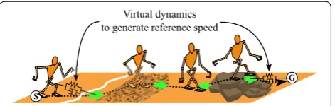
To this end, we challenge this issue by designing vir-tual dynamics between the robot and the goal via a virtual leader point (see Fig. 1). This approach is a com-bination of an artificial potential field concept for mobile robots [14, 15] and a leader-follower formation for mul-tiple agents [16, 17]. Seto and Sugihara have proposed the similar idea for smooth reaching movement [18], but in contrast, our proposal deals with the way to design parameters of the method and optimizes them in real time according to the surroundings. The virtual leader point is attracted to the goal and repulsed by other envi-ronment including obstacles instead of the robot, and consequently, a secure path from the start to the goal is planned autonomously. When the robot follows the leader point within a certain range, the robot reaches the goal while avoiding the obstacles. Such “indirect” interac-tion between the robot and surroundings restrains dras-tic change of the reference gait speeds, namely, they are likely to maintain stability of the current states.
However, this reference generator does not guaran-tee asymptotic stability. Alternatively, more rapid accel-eration would be possible. To ensure asymptotic stability and keep high speed for a long time in pursuit of effi-ciency, the virtual dynamics can be optimized according to a falling risk of the robot by using a selection algorithm for locomotion (SAL) proposed in previous work [19]. SAL optimizes the robot’s mass virtually to maximize an evaluation function, in other words, efficiency within the allowable falling risk, called VM-SAL. Note that unlike previous use of SAL, the evaluation function is difficult to be maximized by the change of the virtual mass. This is because a dominant factor to determine the evaluation function is a set of interaction forces and torques, which are difficult to be optimized freely. To solve this problem, such interaction is regarded as stochastic variable [20],
and instead of the evaluation function, its expected value is maximized.
To evaluate proposed VM-SAL, two types of simula-tions are carried out, while comparing the case without and with VM-SAL. In simulations, the robot achieved the secure and efficient traveling from the start to the goal autonomously. Namely, the robot could travel in the area with obstacles or on a 5° up slope. Specific resistance was fairly small in comparison with walking by a local-stabil-ity-based method conducted in ref. [21].
Our contribution in this paper is not only in system integration from the viewpoint of practicality, but also to expand applicable problems of SAL from the theoretical point of view. Specifically, SAL has solved the optimiza-tion problems for discrete variable using deterministic or stochastic objective [19, 22] and for continuous variables using deterministic objective [19, 23] so far. VM-SAL corresponds to the optimization for continuous variables using stochastic objective, which has not been solved yet. By enabling SAL to cover this problem, most of the opti-mization problems for locomotion can be handled with SAL.
Prerequisites for limit‑cycle‑based bipedal gait and its speed control
Passive dynamic autonomous control: PDAC
Let us introduce a method used as the limit-cycle-based bipedal gait, called passive dynamic autonomous control (PDAC) [21]. PDAC models the robot as an inverted tel-escopic pendulum model, which has a point mass m and three-dimensional half-spherical coordinates (θ,φ,ℓ) , where θ ∈ [0,π/2] means the inclination of the
pendu-lum, φ∈ [−π,π] is for the direction of the inclination,
and ℓ∈(0,∞) gives the pendulum length. Here, ℓ is con-strained by a virtual holonomic constraint (VHC) for robots in accordance with ref. [24], where all joints of the robot interlock with single state variable: in this paper, it is given by θ as ℓ:=ℓ(θ ) . This paper employs the
dynam-ics-based VHC [13] specifically.
By such VHC, the dynamics of the pendulum, θ¨ and φ¨ ,
can be analytically integrated as follows:
(1)
˙
θ (θ ) = ±1
mℓ2(θ )
2
− Cφ
sin2θ+m
2g
ℓ3(θ )sinθdθ+Cθ
= ∓ √
2(−C(θ )+L(θ )+Cθ)
M(θ )
(2)
˙ φ(θ )= ±
2Cφ
mℓ2(θ )sin2θ = ± √
2C(θ )
M(θ )sinθ Fig. 1 Concept of a reference gait speed generator the reference
where g is the gravitational acceleration. Cθ and Cφ are conserved quantities in each gait step, named PDAC con-stants. M(θ ) , C(θ ) , and L(θ ) are substituted for respective terms. In particular, L(θ ) can be solved under the condi-tion that ℓ3(θ )sinθ is integrable. The sign ± in Eq. (2) is
simply chosen by the sign of the initial angular velocity of
φ , φ˙0 . The sign ∓ in Eq. (1) is inverted before and after an
apex.
The bipedal gait exposed by PDAC is fully described by given VHC and two PDAC constants. In particular, the gait speeds are given by the combination of two PDAC constants, whose square roots have the same units of angular momentum.
Adaptive speed controller (ASC)
ASC proposed in the previous work [4] controls the translational (forward and sideward) speeds. Let us intro-duce the principle of ASC. Now, the reference and actual gait speeds are defined as vrefx,yandvx,y , respectively, where x is the forward direction of the robot is facing and y is the sideward direction orthogonal to it. The origin of coordinate system of the swing-leg position pL is on a hip
joint, where is geometrically connected to the vicinity of the center of gravity (COG) position.
Forward speed control
Forward speed control is considered on the basis of shifting an equilibrium point of the robot’s mechani-cal energy. To this end, the momentum of the swing leg is utilized for our solution. As defined in above, PDAC models the robot as the inverted pendulum with a point mass m, but in fact, the mass of the swing leg mL is not
lost as modeling error. The forward swing-up and touch-down positions, psuLx and ptdLx , are simply designed based
on a capture point [25], while the term of the COG posi-tion in the capture point is ignored according to their coordinate system as follows:
where, αx=0.8 is the constant to keep locomotion going forward (or backward), and ω is the natural frequency
of the inverted pendulum ω=g/(ℓ(θ )cosθ ) . ιx is the accumulated term to adapt the swing-up amount for the optimal momentum that yields vrefx .
Sideward speed control
In the bipedal gait, separation of the limit cycles (asym-metric behaviors) for the right and left legs would lead to a slide motion. The degree of this separation is given as the function of the asymmetric touchdown position of (3)
psuLx =(αx+ιx)vxref/ω
(4)
ptdLx =αxv2x/ω
the right and left legs, y , namely, it should be adjusted
to obtain the reference sideward speed. To this end, the sideward touchdown position ptdLy is designed based on the capture point as follows:
where, αy=1.2 is the constant to keep locomotion
stabi-lizing. dL denotes the half of width between the right and
left legs and βL∈ [0, 1] means degree of the vicinity of the
COG. y is adjusted by the integral term ιy to achieve vrefy as well as Eq. (3).
Quasi‑passive dynamic autonomous control (Q‑PDAC) ASC is insufficient to reach arbitrary goal because its sideward speed control is limited depending on the for-ward speed. In that case, the turning speed control is additionally required like a vehicle. We have proposed Q-PDAC in previous work [5] to overcome this problem.
Q-PDAC adds the angular momentum Lw , which is explicitly generated by rotating a yaw-axis hip joint depending on the reference turning speed vwref as follows:
where, Iw is an inertia term and approximated as mdL . 2
Note that the adverse effect of this approximation would be small because the contact position on the ground is basically in the vicinity of the rotating hip joint.
Lw is injected into the PDAC dynamics in Eqs. (1) and (2). The square roots of two PDAC constants, Cθ and Cφ , are the same unit system as the angular momentum. In particular,
2Cφ means the conserved angular momen-tum of φ rotation during one gait step. Thus, Lw can be summed up with
2Cφ in Eq. (2) as follows:
where, the definition of C(θ ) is changed to Eq. (9). In addition, the touchdown position after turning is con-sidered so that v2x and v2y in Eqs. (4) and (5) are
con-verted into the one in coordinate system after turning, respectively.
(5) ptdLy =αyv2y/ω±βLdL−�y
(6)
�y =(αy+ιy)vrefy /ω
(7) Lw=Iwvrefw ≃mdL2vwref
(8)
˙ φ(θ )=±
2Cφ+Lw M(θ )sin2θ
(9)
C(θ ):= Cφ
sin2θ ⇒ (±
2Cφ+Lw)2
Design of virtual dynamics
Overview
The reference gait speeds, the translational speeds vrefx,y
and the turning speed vwref , are generated only from tual attractive (sometimes repulsive) dynamics with a vir-tual leader point. Note that this leader point is regarded as a ghost of the robot, which has the same physical parameters as the robot’s one and goes ahead. The leader point is towed by a goal, while it is repelled by obstacles, such as walls.
Such design of dynamics aims that the robot is indi-rectly towed by the goal and repelled by the obstacles. This indirect interaction yields secure acceleration and deceleration, which are suitable for the limit-cycle-based gait to maintain stability at respective gait speeds, although responsiveness is deteriorated reluctantly.
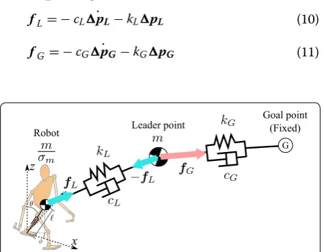
In this section, an attractive force (and torque) between the robot and the leader point, fL (and τL ), and an
attrac-tive force between the leader point and the goal, fG (and τG ), are designed. They entail the secure reference speeds
without falling down at respective gait speeds.
In Appendices A, B, and C, a repulsive force from the obstacles, fO (and τO ), and an explorative force to escape
from stationary points, fE , are defined. Although they are not main focus of this study, they should be imple-mented as a practical matter, as can be seen from many types of previous work [14, 15].
Connection among robot—leader‑point—goal
Above connection model is shown in Fig. 2, where the connections among the robot, the leader point, and the goal, give subscripts L and G. For instance, dampers and springs for their connections are given as cL,G and kL,G
respectively. From these dampers and springs, attractive forces fL and fG are given as follows:
(10) fL= −cLp˙L−kLpL
(11) fG= −cG˙pG−kGpG
where pL and pL˙ are relative distance and velocity between the robot and the leader point, and pG and
˙
pG are relative distance and velocity between the leader point and the goal. Note that attractive torques τL and τG
are given in the same manner. In most cases, fL and fG
are directed to pL and pG , respectively, since trave-ling directions of the robot and the leader point would asymptotically converge to the towing directions.
Given parameters for the connections, namely cL,G and
kL,G , are key parameters to generate the secure reference
gait speeds. Hence, they are designed by giving following intuitive conditions.
Dynamics between leader point and goal
Firstly, the dynamics between the leader point and the goal is designed. To facilitate intuitive comprehension for design, this dynamics is represented by a damping ratio
ζG and a natural angular frequency ωG , instead of cG and
kG.
Now, design criteria are given based on two kinds of time. One is a desired time to arrive at the goal in con-sideration with the robot’s locomotion ability, Ts , and
another is an acceleration time to converge on steady states, Ta . These two are highly easy to be given by
designer.
When Ts is assumed to be a settling time of the
dynam-ics (i.e., the damped oscillation), the leader point will converge on the goal nearly on time.
where es=0.05 means that Ts corresponds to the 5%
settling time. Note that the damped oscillation is rarely settled by Ts since disturbances from the obstacles are
frequently caused.
With respect to Ta , it is assumed to be an inflection point of the dynamics. Namely, Ta is derived by solving equation that the second-order differential of the damped oscillation with ζG <1 is equal to 0.
where tan−1(x) is approximated as x−x3/3 by third-order Maclaurin expansion.
From the above design criteria Ts and Ta , ζG and ωG are
derived as follows:
(12) Ts:=
lnes−1
ζGωG
(13) Ta=
1
ωG
1−ζG2 tan−1
1−ζG2
ζG
≃ Ts lnes−1
1−1−ζ 2 G 3ζG2
cG and kG are derived from ζG and ωG via their
defini-tions: kG=mω2G and; cG=mζGωG . Note that m is
translated into I, which means a moment of inertia, for rotational dynamics.
Now, we focus on the constraint, i.e., Ts≥lnes−1Ta ,
given at deriving ζG . To effectively and surely converge to the goal on time, Ts can be updated every gait step as
Ts←Ts−Tsup , where Tsup means the elapsed time at k-th gait step. Such updating, however, reaches the limi-tation Ts=lnes−1Ta . In that case, ζG becomes 1, and
therefore, the leader point is expected to converge on the goal without oscillation in accordance with the critical damping.
Dynamics between robot and leader point
Secondly, the dynamics between the robot and the leader point is designed. Now, not only cL and kL but also a
damping ratio ζL and a natural angular frequency ωL are
used.
The leader point is required to be naturally in an observable range of the robot, where the robot can observe by a laser sensor or a camera, to allow the robot to avoid the obstacles in surroundings. If the leader point is outside of the observable range, its interaction with the obstacles cannot be calculated. To keep the leader point inside of the observable range, the equilibrium point of fL and fG should be on the edge of the observable range at least. Namely, kL is given from following equilibrium of
fL and fG.
where Robs is the half of radius of maximum observable circle. Note that when the distance between the robot and the leader point meets �pG�2≤Robs , the above condition would be usually kept, namely, kL can be fixed
to kL=kG.
The robot should not become closer to the goal rather than the leader point due to risk of collision with the obstacles. ζL is therefore designed to restrict an
(14)
ζG =
Ts
Ts+3(Ts−lnes−1Ta)
(15) ωG =
lnes−1
ζGTs
(16) kLmax(Robs,�pG�2)−kG�pG�2=0
(17)
∴kL= �pG�2
max(Robs,�pG�2) kG
overshoot of the damped oscillation, in other words, to entail the critical damping, i.e., ζL:=1 . From kL
and ζL , cL is given. Now, as another point of view, the
derivation of kL and ζL sets the settling time of the
dynamics between the robot and the leader point to
Robs/max(Robs,��pG�2)Ts≤Ts . This means that the
robot will converge on the leader point faster than the time when the leader point converges on the goal, and eventually it will converge on the goal by tracking the leader point by Ts.
Design of rotational dynamics between robot and leader point
The above connection models reveal the translational motions of the robot and the leader point. The rotational motions, however, should be treated because the robot cannot travel omni-directional without rotation, as men-tioned above. Hence, the dampers and the springs, which are the same design for translational motions, are con-nected to rotate the leader point and the robot by gener-ating attractive torques τG and τL , respectively. Note that m is replaced with the moment of inertia I in rotation.
Unfortunately, τL is insufficient to reach the leader
point (the goal eventually) in most cases. This is because the sideward speed is absolutely dependent on the for-ward speed, i.e., the bipedal gait is a nonholonomic system similar to wheeled robots. To overcome this limi-tation of the sideward speed, an additional rolimi-tational tor-ques τS is required.
Now, the sideward component of fL is newly divided into fˆL and fS in accordance with the limitation of the
sideward speed. fS is assumed to generate the robot’s
rotation, not translation, and therefore, it is converted into τS as follows:
where tR is the robot’s thickness. In addition, µS∈(0, 1)
is a rotational friction coefficient, and therefore, the rota-tional friction works in the direction depending on the directions of rotational speed and τS : if the direction of τS matches the direction of rotational speed, the friction
direction is given to be minus; otherwise, it is given to be plus.
The leader point receives the reaction force −fS , which
rotates it. Note that the point of load of −fS is regarded as
the rear of the leader point −tR/2 , namely the rotational
torques of the leader point is the same as τS by
cance-ling the sign. This reaction would result in that the robot moves only straight since the attitude error between the (18) τS=(1∓µS)
tR
robot and the leader point becomes equal to 0 and the sideward error also becomes equal to 0.
Update of reference gait speed
The attractive forces, fL (precisely fˆL , which was replaced into fL for simplicity) and fG , and the rota-tional torques, τL , τG , and τS , are given in above sections.
Besides, the force to avoid the obstacles, fO (and τO ), and
the force to escape from the stationary points, fE , are designed in Appendices A, B, and C. Accordingly, the ref-erence gait speed, vref=(vxref,vrefy ,vrefw )⊤ , and the leader
point’s position, pL=(pLx,pLy,pLw)⊤ , are updated under
the influence of them.
Firstly, pL is updated under the condition that all forces
and torques designed in this study act on the leader point.
where dt is a control period at t-th control step.
Secondly, fL , τL , and τS act on the robot to update vref .
While paying attention to a constraint of update timing, when vref can be updated just after touchdown of swing
leg unlike update of pL , vref are updated as follows:
where σm is a variable to adjust the robot’s mass virtually.
The way to adjustment of σm is introduced in next “ Opti-mization of virtual mass by selection algorithm for loco-motion: VM-SAL” section.
Confirmation of convergence
To confirm the convergence of the gait speeds, simple numerical simulations are conducted. In the following simulations, the positions of the leader point and the robot are directly updated according to the given virtual dynamics. First simulations are in one dimension: the goal is in 20 m; the settling time is at 30 s; and a distur-bance ( −5 N) will be injected from 10 to 20 s. Second
(19)
pLx,y[t+1] =pLx,y[t] + ˙pLx,ydt+(−fL+fG+fO+fE)
2m dt
2
(20)
pLw[t+1] =pLw[t] + ˙pLwdt+(−τL+τS2I+τG+τO)dt2
(21) vrefx,y[k+1] =vrefx,y[k] +σmfL
m Tsup
(22)
vrefw [k+1] =vwref[k] +σm(τL+τS)
I Tsup
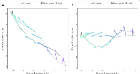
simulations are in three dimensions (x, y, w): two goals are in (10 m, 10 m, 0°) and (0 m, 10 m, 0°); the settling time is at 30 s. The gait speeds converge on the reference gait speeds as given immediately, and the references are updated at about 0.35 s intervals in accordance with the gait step time of the actual robot. σm is fixed to 1. Other
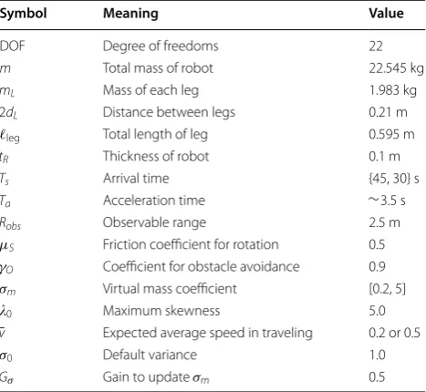
parameters are the same as Table 1.
One‑dimensional simulations
Simulation results are depicted in Fig. 3. When the robot was not disturbed, the robot reached the goal with smooth change of the speed. Even when the robot was disturbed, the robot reached the goal late.
As a remarkable point, the robot accelerated its speed again after the disturbance to catch up. This is the advan-tage of the virtual-dynamics-based (i.e., the state-based) reference speed generator.
Three‑dimensional simulations
Simulation results are depicted in Fig. 4. The robot eventually reached the respective goals in both cases, although their routes were not linear. This is because the sideward speed is limited as mentioned in above.
As a remarkable point, the distance between the robot and the leader point seemed to be so far, although it is in the observable range Robs . If this goes on, the robot would not avoid obstacles due to the tracking delay. This risk comes from no consideration of stability in the design of the virtual dynamics. Therefore, an additional design of
Table 1 Parameters for robot model and proposed method
Symbol Meaning Value
DOF Degree of freedoms 22
m Total mass of robot 22.545 kg
mL Mass of each leg 1.983 kg
2dL Distance between legs 0.21 m
ℓleg Total length of leg 0.595 m
tR Thickness of robot 0.1 m
Ts Arrival time {45, 30} s
Ta Acceleration time ∼ 3.5 s
Robs Observable range 2.5 m
µS Friction coefficient for rotation 0.5
γO Coefficient for obstacle avoidance 0.9
σm Virtual mass coefficient [0.2, 5]
0 Maximum skewness 5.0
¯
v Expected average speed in traveling 0.2 or 0.5
σ0 Default variance 1.0
0 5 10 15 20 25 30 35 40 45
Time [s]
0 5 10 15 20 25
Position [m
]
−0.2 0.0 0.2 0.4 0.6 0.8 1.0
Ve
locity [m
/s
]
Leader point position Robot position
Leader point velocity Robot velocity
0 5 10 15 20 25 30 35 40 45
Time [s]
0 5 10 15 20 25
Position [m
]
Disturbed area
0.0 0.2 0.4 0.6 0.8 1.0
Ve
locity [m
/s
]
Leader point position Robot position
Leader point velocity Robot velocity
a
b
Fig. 3 Examples of the virtual dynamics in one dimension a the robot converged on the goal (20 m) by the settling time (30 s) without disturbance
( −5 N); b even with disturbance, the robot reach the goal late while smoothly changing its speed. a W/O disturbance, b W/ disturbance
0 2
4 6
8 10
Sideward positionpy[m] 0
2 4 6 8 10
Fo
rw
ar
dp
osition
px
[m]
Leader point Follower point (Robot)
0 2
4 6
8 10
Sideward positionpy[m] −6
−4 −2 0 2 4
Forw
ar
dp
osition
px
[m]
Leader point Follower point (Robot)
a
b
σm to ensure asymptotic stability is proposed in the next
section.
Optimization of virtual mass by selection algorithm for locomotion (VM‑SAL)
Overview
We notice that σm changes the robot’s mass virtually so as
to adjust trackability to the leader point. If σm is smaller
than 1, the update of vref is restrained, and such a
behav-ior facilitates the convergence on the limit cycles at cur-rent gait speeds; otherwise, it yields rapid acceleration or deceleration in pursuit of speed or stability. Both of these properties are required, but it is difficult to achieve them simultaneously. In this section, therefore, online optimization of σm by using SAL [19], called VM-SAL, is
explained for secure and efficient bipedal gait.
An unconventional key point to apply SAL to the opti-mization of σm is to estimate an expected value of the
evaluation function, which is maximized by optimiz-ing σm . This is because a main factor for the evaluation
function is stochastically given by the virtual dynamics designed in above, and σm determines just a tendency of
its dynamics.
Selection algorithm for locomotion
In general, locomotion has a trade-off relation between stability and efficiency (e.g., energy efficiency and gait speed). Several approaches to select locomotion, there-fore, have been proposed for switching the priority of stability and efficiency according to the situation [19, 26,
27]. SAL is the state-of-the-art algorithm among those approaches. SAL is divided into two phases: a recogni-tion phase and a selecrecogni-tion phase (see ref. [19] for more details).
In the recognition phase, the robot estimates the many uncertainties for locomotion from sensors: in this paper, zero moment point (ZMP) errors on x- and y-axes; a touchdown timing error; a swing-leg trajectory error; a step height; and a slope angle. They are integrated sto-chastically as a falling risk S using a Bayesian network. The structure of the Bayesian network and the connec-tion strength between the nodes are obtained via offline and online learning.
As reported in ref. [19], S is proportional to the change of the gait speed v . The gait-speed-based falling risk Sv is therefore defined as follows:
where Cv is a coefficient, although it is simplified as 1. In the selection phase, the robot reveals the desired balance of stability and efficiency, and adjusts the bal-ance toward the desired one by changing its variables of locomotion. Here, the desired balance of stability (23)
Sv:=S+Cvv
and efficiency is defined the maximum efficiency within allowable falling risk (in most cases, without falling down). The variable is given as σm in this paper (see the
next section).
To satisfy the desired balance of stability and efficiency, locomotion reward R is defined by product of a smooth threshold of the allowable falling risk and the efficiency given as a linear combination of the gait speed v and a reciprocal of specific resistance (or cost of transport)
1/Cmt [28].
where CR1=100 and CR2=20 are coefficients used to adjust the priority between v and Cmt . t is the current time step, and N=5 is the maximum time step used for predicting the falling risk. Further, r designs the shape of the logistic function. γS=0.8 is the reliability of the
pre-diction and γSreg is a normalization term.
Assumption for interaction forces as stochastic variables Maximization of R yields the desired balance of stabil-ity and efficiency for locomotion. The virtual mass vari-able σm is therefore newly optimized for the purpose of
maximization of R. Now, the role of σm has appeared in
Eqs. (21) and (22): large/small σm strengthens/weakens
the influences of given interaction forces and torques. In other words, σm can adjust v in SAL indirectly.
However, dominant factors for v are obviously the
interaction forces and torques, fL , τL , and τS , and
there-fore, the effect of σm for R highly depends on them. This
means that σm would oscillate if it is optimized by
previ-ous SAL, which decides optimal values deterministically. To solve this problem, the interaction forces and tor-ques are regarded as stochastic variables: i.e., v is also
regarded as a stochastic variable. In general, when the gait speed v is under the average speed to travel from the start to the goal by Ts , namely v¯ , v tends to be
posi-tive to accelerate; otherwise, v tends to be negative to
decelerate. Hence, v has a skewness depending on v in
its distribution.
To represent this skewness, v is assumed to be
follow-ing skew normal distribution SN proposed in ref. [20].
where v is replaced as x for the sake of convenience. φ is the standard normal probability density function with
(24) R:=
1−γSreg
N
n=0
γSn 1+er(1/2−S(t+n))
CR1v+ CR2 Cmt
(25) �v:=x∼SN(µ,σ,)
=σ2φ
x−µ σ
�
x−µ
its cumulative distribution function . This SN has three parameters that should be given: a location µ ; a scale σ ; and a shape . From these three, its mean µskew , its vari-ance σskew , and its skewness γskew are derived.
Now, these three parameters, µ , σ , and are designed according to the behavior of v . For the sake of conveni-ence, δ is defined as follows:
where δ is within [0,√2/π ).
With respect to µ , it is simply designed to be 0. In that
case, µskew is given to be µskew=σ δ.
We can easily assume that σ correlates with σm since v is proportional to σm . σ is, however, not actual variance of SN , which is absolutely proportional to σm . Thus, the relation between σ and σm is given via σskew as follows:
where σ0 is default variance of SN.
Finally, is designed to represent the dependency on v. (26)
δ():=
2 π
√
1+2
(27)
σskew=σ0σm=σ
1−δ2
∴σ =
σ0σm
√ 1−δ2
(28) (v):=0
1−v
¯
v
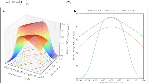
where 0 is an initial skewness at v=0 . The case with 0=5 and ¯v=0.5 is illustrated in Fig. 5.
Maximization of expected value of locomotion reward From the above skew normal distribution, the expected value of R, namely ER , can be derived as follows:
Note that this integral is hard to calculate analytically.
R is therefore approximated by third-order Maclaurin expansion, which gives an analytical solution according to properties of probability distribution by using µskew ,
σskew , and γskew . Here, η0–3 means 0–3-th order terms of
R regarding σm.
To maximize ER , the virtual mass factor σm is
opti-mized by using SAL, called VM-SAL. This purpose can be achieved by using the gradient of ER with respect to
(29) ER(σm) =
∞
−∞
R(x)SN(0,σ (σm),)dx
(30) ≃
∞
−∞
(η0+η1x+η2x2+η3x3)SN(0,σ (σm),)dx
(31) =η0+η1µskew+η2(σskew2 +µ2skew)
+η3(γskewσskew3 +3µskewσskew2 +µ3skew)
Next
gait speed: v+ ∆
v −0.50
−0.250 .000.25
0.500.75 1.001
.251 .50
Gait speed:
v
0.0
0.2 0.4
0.6
0.8
1.0 Densi
ty
:SN (µ,σ (σm ,λ)
,λ
(
v))
0.0 0.1 0.2 0.3 0.4 0.5
−0.50 −0.25 0.00 0.25 0.50 0.75 1.00 1.25 1.50
Next gait speed:v+ ∆v 0.0
0.1
0.2 0.3 0.4
0.5
Densit
y:
SN
(
µ,
σ
(
σm
,λ
)
,λ
(
v
))
v= 0.0 v= 0.5 v= 1.0
a
b
Fig. 5 Skewness of SN depending on v when v is smaller than v¯=0.5 , the skewness is plus since the dynamics tends to accelerate v; otherwise, it
σm , ∂ER/∂σm . Namely, σm should be updated according to the direction of the gradient as follows:
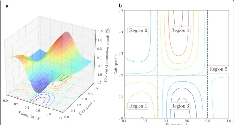
where Gσ is a gain. The gradient is normalized by its max-imum value (it would be at v=2v¯ and S=0.5).
One typical sample of the gradient, which has σm=1 and other parameters are the same as Table 1, is illus-trated in Fig. 6. The gradient in Fig. 6 is divided into five regions to determine the behavior of VM-SAL.
1. Stable state with low speed (the gradient is plus): the robot would accelerate rapidly to get high speed. 2. Stable state with high speed (the gradient is minus):
the robot would keep high speed for efficiency to reach the goal fast.
3. Unstable state with low speed (the gradient is minus): the robot would keep low speed for stability not to fall down.
4. Unstable state with high speed (the gradient is plus): the robot would decelerate rapidly to travel carefully. 5. Highly unstable state (the gradient is almost zero):
this region would be out of scope of VM-SAL. (32)
σm[k+1] =σm[k] +Gσ
max∂ER ∂σm
−1 ∂ER ∂σm
These behaviors are certainly reasonable similar to human behaviors, although they are absolutely deter-mined based on the expected value. Namely, we notice that they would not be always expected.
Simulation
Simulation conditions Robot details
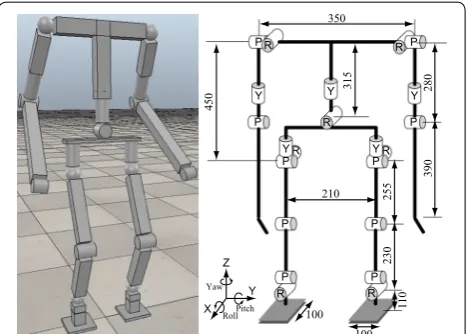
Following two types of simulations are conducted on a simulator named V-REP [29]. An using robot model is created based on Gorilla Robot III that has been devel-oped for a prototype of multi-locomotion robot [13,
30], as shown in Fig. 7. This model measures whole joint angles by respective encoders, and three-axis angu-lar velocities by a gyro sensor mounted on the torso, and three-axis acceleration by an acceleration sensor mounted on the torso. They are used to predict the cur-rent COG states. In addition, the environmental map is given in advance, and a laser sensor is assumed to be used to estimate the self location. A contact model between the ground and the foot of the robot is defined as a non-slip model, and to this end, the COG trajec-tory is forcibly modified under the limitation of the fric-tion pyramid and gravitafric-tional accelerafric-tion. From the COG trajectory and the swing leg trajectory, the resolved momentum control [9] generates whole joint angles,
Falling risk:S 0.0
0.2 0.4
0.6 0.8
1.0 Ga
itsp eed:
v
0.0 0.1
0.2 0.3
0.4 0.5
:d
ra
wer
noi
to
mo
col
fo
tn
ei
dar
G
∂
ER ∂σm
−1.5 −1.0 −0.5 0.0 0.5 1.0 1.5
0.0 0.2 0.4 0.6 0.8 1.0
Falling risk:S 0.0
0.1 0.2 0.3 0.4 0.5
Gait
sp
eed:
v
Region 1 Region 2
Region 3 Region 4
Region 5
a
b
which are kinematically obtained almost exactly. Note that the above calculation time to generate whole joint angles was confirmed to be less than 1 ms by Intel Core i7 (2.2 GHz), which is the control step time in the following simulations.
Parameters for the robot model and proposed method are summarized in Table 1. Note that torque and angu-lar velocity of all joints are almost limitless for simplic-ity. Now, the gait speed is represented by a dimensionless format, i.e., a Froude number Frd calculated by v/
gℓleg
( ℓleg is a leg length).
Environment details
In the first type of simulation, the robot will go toward the goal: (px,py,pw)= (15 m, 15 m, 90°). In the middle of traveling, four pillars are arranged as obstacles to dis-turb traveling. This simulation is desired to be finished by Ts=45 s, namely, v¯ is derived to be about 0.2.
In the second type of simulation, the robot will go straight toward the goal: (px,py,pw)= (25 m, 0 m, 0°). The settling time is given as Ts=30 s, namely, v¯ is derived to
be about 0.5. When the gait speed of our robot model is over 0.5, the gait will transit to running in pursuit of energy minimization [13, 31], although running is easy to break its balance [32]. A slope with 5° inclination is set on the way, and therefore, the robot should transit to walk-ing again for secureness.
In both types, two cases, without and with VM-SAL, are compared to evaluate the performance of VM-SAL. In terms of secure traveling, a distance between the robot and the leader point or a phase of the gait formed by (θ,θ˙,φ)˙ is confirmed. In terms of efficient traveling, the specific resistance Cmt [28] is evaluated.
The above simulations are finished as successful cases when the robot steps into the radius of 0.5 m of the goal at a stopable gait speed ( |Frd|<0.1 ). This stopable gait speed was given from experience of experiments and simulations so far. In failure cases, the COG trajectory cannot be generated by PDAC due to the infeasible initial parameters, and the robot would fall down eventually.
Simulation results
All simulations were recorded in the attached video. In the following, effectiveness of VM-SAL is verified from the simulation results (Additional file 1).
Traveling while avoiding obstacles
Geometric trajectories from the start to the goal, ZMP margins, and forward gait speeds were depicted in Figs. 8,
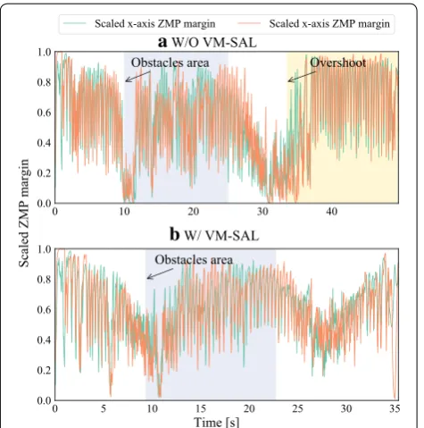
9, and 10, respectively. In both cases, the robot reached the goal while avoiding the obstacles, although the case without VM-SAL sometimes had the ZMP on the edge of the support polygons, namely it might be failed to keep the dynamic constraints. In first and last areas (i.e., sta-ble areas), VM-SAL yielded the rapid acceleration rather than the case without VM-SAL for efficiency. In the obstacles area, VM-SAL decreased the gait speed and kept it low for secureness since locomotion was slightly deviated from steady walking to avoid the obstacles, and that caused increase of the falling risk.
As can be seen in these figures, in the case with-out VM-SAL, the robot went through the goal due to Fig. 7 Modified model of Gorilla Robot III for simulation its weight is
about 22 kg; its height is about 1 m; total DOFs are given as 22
0 5
10 15
Sideward position py [m] 0
5 10 15
Forward position
px
[m
]
Start Goal: W/O=49.6 s, W/=35.4 s
Robot W/O VM-SAL
Leader point W/O VM-SAL Robot W/ VM-SALLeader point W/ VM-SAL
insufficient brake, while in the case with VM-SAL, the robot could stop near the goal on the first attempt. As a result, respective arrival times were highly different: 49.6 s in the case without VM-SAL; and 35.4 s in the case with VM-SAL.
To confirm the behavior of VM-SAL, observed data were plotted in Fig. 11. The change of σm was confirmed as intended, although the behavior resulting from it was not always as expected. In the obstacles area (i.e., the region 4), σm became large for secure traveling, and actu-ally, the gait speed was decelerated. The mean σm was large, 4.6, since the robot’s state was not stepped in the regions 2 and 3 deeply. This is due to influence of insta-bility by high speed and weak disturbance by obstacles. Such large σm instead enabled to stop on the goal as a result, although it is expected to achieve high speed.
Two types of indexes were evaluated in addition to the arrival time (see Fig. 12): the distances between the robot and the leader point (�r,�θ ) for secureness; and the spe-cific resistance Cmt for efficiency. Keeping the distances
short yields the gradual update of the gait speeds, which would reduce the risk of falling down by large accelera-tion/deceleration. Conversely, σm optimized by VM-SAL tends to make (�r,�θ ) small. Furthermore, such secure acceleration and deceleration yielded rapid convergence to the steady state, namely Cmt became small about half.
Traveling on slope
Time-series data of ZMP margins and the reference and actual gait speeds were depicted in Figs. 13 and 14. In both cases, the gait transited to running when its speed was over 0.5, while keeping ZMP in the support polygons.
0 10 20 30 40
0.0 0.2 0.4 0.6 0.8 1.0
Obstacles area Overshoot Scaled x-axis ZMP margin Scaled x-axis ZMP margin
0 5 10 15 20 25 30 35 0.0
0.2 0.4 0.6 0.8 1.0
Obstacles area
Time [s]
Scaled ZMP margi
n
a
W/O VM-SALb
W/ VM-SALFig. 9 ZMP margin scaled by the maximum distance to the edge of the support polygons a when stepping into the obstacle area, the robot was disturbed by the obstacles, and ZMP was instantaneously on the edge of the support polygons; b the robot succeeded to keep ZMP in the support polygons
a
b
Fig. 10 Reference and actual forward gait speed a even in the obstacles area, the gait speed was hardly decreased, which caused oscillation of actual gait speed; the robot could not brake its speed on the goal, and wasted about 16 s to reach the goal; b in the first stable area, the gait speed was rapidly accelerated to prioritize efficiency; in the obstacles area, the robot braked to prioritize stability
Fig. 11 Verification of behavior of VM-SAL the plotted data has
the size based on σm−1 and the color based on the change of σm ;
in the region 4 with above-average speed and high falling risk (i.e.,
when initial stage in the obstacles area), σm became large to easily
decelerate for stability; in the middle of and after the obstacles area,
excess increase of σm was restrained due to above-average speed and
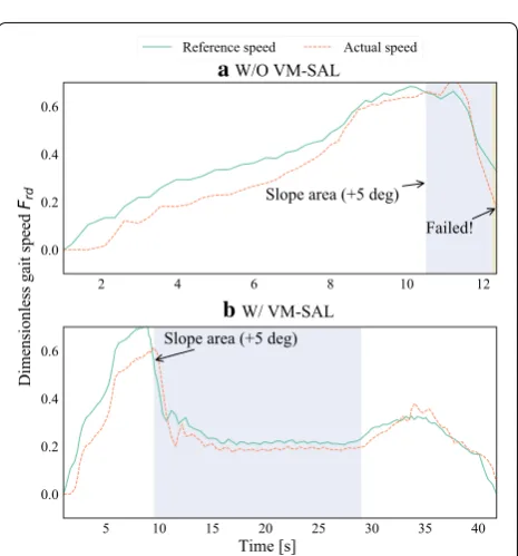
The robot failed to travel on the slope in the case without VM-SAL due to delayed deceleration to transit to walk-ing. In contrast, the robot started to decelerate the gait speed rapidly before stepping into the slope in the case with VM-SAL. Consequently, the robot succeeded in reaching the goal beyond the slope.
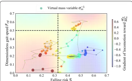
To confirm the behavior of VM-SAL, observed data were plotted in Fig. 15. A notable difference from trave-ling in the area with obstacles shown in Fig. 11 appeared in the slope area. Namely, the gait speed was decelerated but the slope kept the falling risk high, and therefore, σm became smaller than 1 in the region 3. Small σm pre-vented disturbance caused by unnecessary acceleration and deceleration. This behavior yielded the secureness to succeed in going through the slope, although the arrival time was delayed by about 10 s.
Two indexes were evaluated in addition to the arrival time (see Fig. 16): the phase formed by (θ,θ˙,φ)˙ to confirm
a
b
Fig. 12 Evaluation of secureness and efficiency both indexes are improved about twice by VM-SAL. a Distance between the robot and the leader point. b Specific resistance in related to the gait speed
0 2 4 6 8 10 12
0.0 0.2 0.4 0.6 0.8 1.0
Slope area (+5 deg)
Failed!
Scaled x-axis ZMP margin Scaled x-axis ZMP margin
0 5 10 15 20 25 30 35 40 0.0
0.2 0.4 0.6 0.8 1.0
Slope area (+5 deg)
Time [s]
Scaled ZMP margi
n
a
W/O VM-SALb
W/ VM-SALFig. 13 ZMP margin scaled by the maximum distance to the edge of the support polygons In both cases, ZMP could be kept in the support polygons, although its margin was small when the robot ran; a in the case without VM-SAL, the robot could not keep its balance on the slope and failed; b in the case with VM-SAL, even on the slope, the robot got steady walking and ZMP also became stable
a
b
asymptotic stability; and the specific resistance Cmt for
effi-ciency. As can be seen in the phase, the respective gaits (walking on flat, walking on slope, and running) converge to respective limit cycles, namely, asymptotic stability could be judged to be guaranteed. On the other hand, the case without VM-SAL (on slope) could not converge to specific limit cycle, and the COG trajectory was failed to be generated by PDAC. Larger Cmt than the case without
VM-SAL (this data was evaluated until falling) was due to influence of the slope, where potential energy was addition-ally required. Even in consideration of that point, the case with VM-SAL achieved fairly good efficiency in compari-son with walking on flat by a local-stability-based method conducted in ref. [21] ( Cmt=0.57 by the actual robot).
Conclusion
In this paper, we achieved the secure and efficient refer-ence gait speed generator, i.e., the virtual dynamics with VM-SAL. The virtual dynamics was given among the robot—the leader point—the goal, and designed based on the desired time to arrive at the goal, Ts , and the
accelera-tion time, Ta . Namely, this dynamics enabled the robot to reach the goal on time implicitly if no disturbances were added. The reference gait speeds were generated from this dynamics, however, they did not always maintain the limit cycle at respective gait speeds. Alternatively, more rapid acceleration and deceleration would be possible.
To ensure asymptotic stability and enhance efficiency, SAL optimizes the robot’s mass virtually depending on the gait speed and the falling risk, called VM-SAL. This VM-SAL aimed to maximize the locomotion reward sto-chastically. Namely, its expected value was maximized by updating the virtual mass variable σm in accordance with its gradient.
As a result, the robot traveled from the start to the goal in two types of environment: one is with the four pillars as obstacles; another is with the 5° up slope. When the robot traveled in the area with these obstacles, VM-SAL improved both trackability (i.e., secureness) and the spe-cific resistance (i.e., efficiency) doubled in comparison with the case without VM-SAL. When the robot traveled on the slope, VM-SAL achieved rapid transition between walking and running according to the gait speed and pre-vented disturbance caused by unnecessary acceleration and deceleration. Such transition succeeded in traveling even though the case without VM-SAL failed to travel.
To regard v as the stochastic variable shown in Fig. 5 is a fairly rough assumption, which would cause unex-pected behaviors. Future challenge of this research is therefore to reflect observed data into parameters of the stochastic variable for more effective optimization of σm . Such reflection restrains the behavior contrary to expectation.
Fig. 15 Verification of behavior of VM-SAL the plotted data has the
size based on σm−1 and the color based on the change of σm ; on the
slope, the state was kept in the region 3 to prevent speed fluctuation; the region 2 was hardly visited because running with high speed tends to be risky
a
b
Fig. 16 Evaluation of secureness and efficiency a all gaits with VM-SAL achieved respective limit cycles, while the case without VM-SAL (on slope) failed to converge to specific limit cycle; b slightly
high Cmt included potential energy to go up the slope. a Phase
Additional file
Additional file 1. Simulation videos: the robot of gray/wine color are with/without VM-SAL, respectively; in two scenarios, VM-SAL improved the gait stability and efficiency and enabled the robot to stop on the given goals smoothly.
Authors’ contributions
TF, YH, and KS designed and directed the project. TK and TA processed the experimental data, performed the analysis, drafted the manuscript. All authors read and approved the final manuscript.
Author details
1 Division of Information Science, Nara Institute of Science and Technology,
8916-5 Takayama, Ikoma, Nara 630-0192, Japan. 2 Department of Micro-Nano
Mechanical Science and Engineering, Nagoya University, Nagoya, Japan.
3 Faculty of Science and Engineering, Meijo University, Nagoya, Japan. 4
Intel-ligent Robotics Institute, School of Mechatronic Engineering, Beijing Institute of Technology, Beijing, China.
Acknowledgements
This work was supported by JSPS KAKENHI, Grant-in-Aid for JSPS Fellows, Grant Number 16J05354.
Competing interests
The authors declare that they have no competing interests.
Publisher’s Note
Springer Nature remains neutral with regard to jurisdictional claims in pub-lished maps and institutional affiliations.
Appendix
Appendix A: Avoidance of obstacles
To avoid obstacles, many studies [14, 15] deal with vir-tual repulsive forces from obstacles to the robot. In limit-cycle-based bipedal gait, however, such repulsive forces may deviate the robot’s state from the limit cycle to guarantee stability, thereby causing falling down. This problem can be solved by indirect interaction with the obstacles by means of the leader point, as mentioned in “Overview” section.
Here, the obstacles generating the repulsive forces are restricted to the ones that are in the circle around the leader point with Robs radius. If Eq. (17) is properly sat-isfied, this circle would fit into the maximum observable range of the robot. This restriction reduces calculation cost, while ensuring the minimum necessary number of the obstacles.
The repulsive force generated by the i-th observed obstacle Oi , fi , is assumed to be inversely proportional
to the square of the distance between Oi and the leader
point, ri , and the masses of both, mi and m. ri is given as
Mahalanobis distance calculated using major and minor axes of the ellipse covering Oi , ai and bi , as shown in
Fig. 17a.
(33)
ri=
pix bi
2 +
piy ai
2
where pi =(pix,piy)⊤ is the leader point’s position
rela-tive to the coordinate of Oi . The coordinate of Oi defines its origin on the point, where the leader point may col-lide, and the y axis as the major axis of the ellipse.
Now, the way to design mi and a constant of
propor-tionality Gi is introduced, although they have been
designed experimentally in almost cases of previous stud-ies. This study focuses on kinetic energy by the velocity of the leader point approaching to Oi , given vi . Note that vi
is divided into three cases: whether the actual velocity of the leader point vL=(vLx,vyL)⊤ intersects Oi ; whether vL
intersects the y axis of Oi ; and whether vL is not directed
to Oi.
a
b
The kinetic energy produced by vi should be converted into the potential energy stored by the repulsive force field not to collide with Oi . The conversion to the poten-tial energy would be started just after the observation of Oi . The farthest distance at starting the observation is assumed to be Robs/bi . If conversion to the potential
energy is finished at γORobs/bi , where γO ∈(0, 1) is an
appropriate magnification, mi and Gi are derived together
from the relation between the kinetic and potential energy.
Even when the observation is started at Robs/ai , which means the closest case, with this design, the kinetic energy is converted into the potential energy since the repulsive force becomes stronger than the farthest case.
From the above, total of the repulsive forces, fO , is given as follows:
where NO is the number of the obstacles in the
observ-able range of the robot.
Appendix B: Rotational torque to contour lines of the gradient
To facilitate avoidance of obstacles and escape from sta-tionary points, it is effective to rotate the attitude of the leader point toward contour lines of the gradient gener-ated by obstacles, as can be seen in Appendix C. Such rotation is assumed to be completed in time TO , when
momentum of the leader point will be consumed by the repulsive force fO . Finally, the leader point is rotated by (34) vi=
�vL�2 | −v
L y
vL
xpix+piy| ≤ai
vL·(−pi) �pi�2 | −
vL y
vL
xpix+piy|>ai
0 − v
L y
vL x ≥0
(35)
1 2mv
2 i =
γORobsbi
Robs bi
−Gi
mmi
ri2 dr=Gimmi 1−γO
γO bi Robs
(36)
∴Gimi =1 2
γO 1−γO
Robs bi
v2i
(37) fO=
NO
i=1
fi= −mRobs
2 γO
1−γO NO
i=1 v2i biri2
dynamics of critical damping, which is designed on the basis of settling time TO.
Before considering the momentum of the leader point, an average force of fO , f¯O , is derived from the relation
between work and energy. Namely, fO is assumed as a non-conservative force. f¯O is derived according to this
assumption as follows:
where the minus sign in right-hand side of above equa-tion is given since fO is the repulsive force.
¯
fO can be converted into an impulse f¯OTO , which is
allowed to dissipate the momentum of the leader point. Namely, TO is derived from law of conservation of
momentum as follows:
By regarding TO as the settling time of the critical
damp-ing, a damper cO and a spring kO , which are connected
between the leader point and the contour line for con-vergence destination, are given as well as cL,G and kL,G .
The rotational torque τO is generated from cO and kO as
follows:
where pOw and ˙pO
w are angular difference and its
veloc-ity between the leader point and the contour line. Note that the direction of τO , in other words which direction
of the contour line becomes targeted, is in accordance with the direction close to a current attitude of the leader point.
Appendix C: Escape from stationary points
As a drawback of the dynamics-based reference genera-tors, such as an artificial potential field approach, station-ary points would be caused from equilibrium of acting forces (i.e., −fL , fG , and fO ). The leader point should escape from such stationary points by adding an explora-tive force fE . Note that the robot (i.e., the reference gait speeds) does not requrie the explorative force since the (38)
1 2mv
2
O= − ¯fO(1−γO)Robs
∴f¯O= −1 2mv
2
O 1 (1−γO)Robs
(39)
0−mvO= ¯fOTO
∴ TO= − mvO
¯
fO
= 2(1−γO)Robs
vO
robot is towed only by the leader point, namely no sta-tionary points are caused.
fE is generated based on the attractive force fG (see Fig. 17b). Firstly, a required level of fE , named E , should be considered. When the equilibrium of acting forces occurs, its dominant forces are estimated as fG and fO . Namely, if fG and fO are not similar vectors to each other, in particular vectors in the opposite direction, fE is required. E is therefore given as a cosine similarity between fG and fO.
where E is in the range of [0, 1]. When fG and f
O are
opposite vectors to each other, E is fixed to be equal to 1. Secondly, a direction of fE should be considered. This direction is basically given as a tangential direction of the contour lines of fO so as to minimize fO while avoid-ing the obstacles. The leader point is rotated along to the contour lines, hence, the direction of fE is reasonably given to be the attitude of the leader point pLw.
fE is therefore designed as follows:
where ERG is a rotational matrix from the direction of fG to pLw.
If part of fG is assumed to be converted into fE , fG is modified as follows:
Publisher’s Note
Springer Nature remains neutral with regard to jurisdictional claims in pub-lished maps and institutional affiliations.
Received: 11 February 2018 Accepted: 17 August 2018
References
1. McGeer T (1990) Passive dynamic walking. Int J Robot Res 9:62–82 2. Hobbelen DGE, Wisse M (2008) Controlling the walking speed in limit
cycle walking. Int J Robot Res 27(9):989–1005
3. Luo X, Zhu L, Xia L (2015) Principle and method of speed control for dynamic walking biped robots. Robot Auton Syst 66:129–144 4. Kobayashi T, Aoyama T, Hasegawa Y, Sekiyama K, Fukuda T (2016)
Adap-tive speed controller using swing leg motion for 3-D limit-cycle-based bipedal gait. Nonlinear Dyn 84(4):2285–2304
5. Kobayashi T, Sekiyama K, Hasegawa Y, Aoyama T, Fukuda T (2016) Quasi-passive dynamic autonomous control to enhance horizontal and turning gait speed control. In: IEEE/RSJ international conference on intelligent robots and systems, pp 5612–5617
6. Gregg RD, Righetti L (2013) Controlled reduction with unactuated cyclic variables: application to 3d bipedal walking with passive yaw rotation. IEEE Trans Autom Control 58(10):2679–2685
(41) E =
1− fG·fO
�fG�2�fO�2 fG·fO>0
1 otherwise
(42) fE =ERGEfG
(43) fG⇐(1−E)f
G
7. Gregg RD, Tilton AK, Candido S, Bretl T, Spong MW (2012) Control and planning of 3-d dynamic walking with asymptotically stable gait primi-tives. IEEE Trans Robot 28(6):1415–1423
8. Kajita S, Kanehiro F, Kaneko K, Fujiwara K, Yokoi K, Hirukawa H (2003) Biped walking pattern generation by a simple three-dimensional inverted pendulum model. Adv Robot 17(2):131–147
9. Kajita S, Kanehiro F, Kaneko K, Fujiwara K, Harada K, Yokoi K, Hirukawa H (2003) Resolved momentum control: humanoid motion planning based on the linear and angular momentum. IEEE/RSJ Int Conf Intell Robots Syst 2:1644–1650
10. Kuffner J, Nishiwaki K, Kagami S, Inaba M, Inoue H (2005) Motion plan-ning for humanoid robots. Robot Res 15:365–374
11. Perrin N, Stasse O, Baudouin L, Lamiraux F, Yoshida E (2012) Fast human-oid robot collision-free footstep planning using swept volume approxi-mations. IEEE Trans Robot 28(2):427–439
12. Gregg RD, Spong MW (2010) Reduction-based control of three-dimen-sional bipedal walking robots. Int J Robot Res 29(6):680–702
13. Kobayashi T, Sekiyama Y, Hasegawa Y, Aoyama T, Fukuda T (2018) Unified bipedal gait for autonomous transition between walking and running in pursuit of energy minimization. Robot Auton Syst 103:27–41
14. Khatib O (1986) Real-time obstacle avoidance for manipulators and mobile robots. Int J Robot Res 5(1):90–98
15. Deng M, Inoue A, Sekiguchi K, Jiang L (2010) Two-wheeled mobile robot motion control in dynamic environments. Robot Comput Integrated Manuf 26(3):268–272
16. Das AK, Fierro R, Kumar V, Ostrowski JP, Spletzer J, Taylor CJ (2002) A vision-based formation control framework. IEEE Trans Robot Autom 18(5):813–825
17. Asl AN, Menhaj MB, Sajedin A (2014) Control of leader-follower formation and path planning of mobile robots using asexual reproduction optimi-zation (ARO). Appl Soft Comput 14:563–576
18. Seto F, Sugihara T (2010) Motion control with slow and rapid adaptation for smooth reaching movement under external force disturbance. In: IEEE/RSJ international conference on intelligent robots and systems, pp 1650–1655 19. Kobayashi T, Aoyama T, Sekiyama K, Fukuda T (2015) Selection algorithm for locomotion based on the evaluation of falling risk. IEEE Trans Robot 31(3):750–765
20. Azzalini A (1985) A class of distributions which includes the normal ones. Scand J Stat 12(2):171–178
21. Aoyama T, Hasegawa Y, Sekiyama K, Fukuda T (2009) Stabilizing and direc-tion control of efficient 3-D biped walking based on PDAC. IEEE/ASME Trans Mech 14(6):712–718
22. Kobayashi T, Sekiyama K, Aoyama T, Fukuda T (2015) Cane-supported walking by humanoid robot and falling-factor-based optimal cane usage selection. Robot Auton Syst 68:21–35
23. Kobayashi T, Sekiyama K, Aoyama T, Hasegawa Y, Fukuda T (2016) Selec-tion of two arm-swing strategies for bipedal walking to enhance both stability and efficiency. Adv Robot 30(6):386–401
24. Grizzle JW, Abba G, Plestan F (2001) Asymptotically stable walking for biped robots: analysis via systems with impulse effects. IEEE Trans Autom Control 46(1):51–64
25. Pratt J, Carff J, Drakunov S, Goswami A (2006) Capture point: a step toward humanoid push recovery. In: IEEE-RAS international conference on humanoid robot, pp 200–207
26. Toda K, Tomiyama K (2007) An adaptive biped gait generation scheme utilizing characteristics of various gaits. In: Humanoid robots, human-like machines, InTech, New York, pp 228–244
27. Saglam CO, Byl K (2014) Quantifying the trade-offs between stability versus energy use for under actuated biped walking. In: IEEE/RSJ interna-tional conference on intelligent robots and systems, pp 2550–2557 28. Collins S, Ruina A, Tedrake R, Wisse M (2005) Efficient bipedal robots
based on passive-dynamic walkers. Science 307:1082–1085 29. Rohmer E, Singh SPN, Freese M (2013) V-REP: a versatile and scalable
robot simulation framework. In: IEEE/RSJ international conference on intelligent robots and systems, pp 1321–1326
30. Fukuda T, Hasegawa Y, Sekiyama K (2012) Multi-locomotion robotic systems: new concepts of bio-inspired robotics. Springer, Berlin 31. Srinivasan M, Ruina A (2006) Computer optimization of a minimal biped
model discovers walking and running. Nature 439(5):72–75 32. Seipel JE, Holmes P (2005) Running in three dimensions: analysis of a