The Best Approximation of the Sinc Function by a Polynomial of Degree with the Square Norm

Volume 2010, Article ID 307892,12pages doi:10.1155/2010/307892

Research Article

The Best Approximation of the Sinc Function by

a Polynomial of Degree

n

with the Square Norm

Yuyang Qiu and Ling Zhu

College of Statistics and Mathematics, Zhejiang Gongshang University, Hangzhou 310018, China

Correspondence should be addressed to Yuyang Qiu,[email protected]

Received 9 April 2010; Accepted 31 August 2010

Academic Editor: Wing-Sum Cheung

Copyrightq2010 Y. Qiu and L. Zhu. This is an open access article distributed under the Creative Commons Attribution License, which permits unrestricted use, distribution, and reproduction in any medium, provided the original work is properly cited.

The polynomial of degreenwhich is the best approximation of the sinc function on the interval0,

π/2with the square norm is considered. By using Lagrange’s method of multipliers, we construct the polynomial explicitly. This method is also generalized to the continuous function on the closed intervala, b. Numerical examples are given to show the effectiveness.

1. Introduction

Let sincx sinx/x be the sinc function; the following result is known as Jordan inequality1:

2

π ≤sincx<1,0< x≤ π

2, 1.1

where the left-handed equality holds if and only ifxπ/2. This inequality has been further refined by many scholars in the past few years2–30. ¨Ozban12presented a new lower bound for the sinc function and obtained the following inequality:

2

π

1

π3

π2−4x24π−3 π3

x−π

2 2

≤sin cx. 1.2

The above inequality was generalized to an upper bound by Zhu26:

sin cx≤ 2

π

1

π3

π2−4x212−π

2

π3

x− π

2 2

Later, Agarwal and his collaborators2proposed a more refined two-sided inequality:

1−4

−6643π−7π2

π2 x−

4124−83π14π2

π3 x

2₋412−4π

π4 x

3

≤sin cx≤1−4

−7549π−8π2

π2 x

4−14295π−16π2

π3 x

2₋412−4π

π4 x

3_,

1.4

where the two-sided equalities hold ifxtends to zero orxπ/2.

Note that the bounds of the sinc function sincx listed above are estimated by the given polynomials with the boundary constraints; the smaller the residual between the polynomial and the sinc function is, the more refined the estimation will be. Hence, our aim is to seek a polynomial of degreen,pnx, which is the best approximation of the sinc function

with the square norm. In view of that, the sinc function is defined on 0, π/2 and two boundary constrained conditions are imposed. So we want to solve the following minimum problem:

min

pnx∈Pn

π/2

0

sin cx−pnx

2 dx

1/2

s.t. lim

x→0pnx _xlim_→0sin cx, _x→lim_π/2pnx _x→lim_π/2sincx,

1.5

wherePnis the set of the polynomial of degreenand it is denoted by

Pn pn|pnx a0a1x· · ·anxn, ai∈R, i1,2, . . . , n

1.6

In this paper, an explicit representation for the approximating polynomial of sincx is presented by using Lagrange’s method of multipliers, and numerical examples are given to show the effectiveness. Moreover, this method can be generalized to the continuous function

gxon the closed interval a, b. However, the residual error between the approximating polynomialpnxandgxis concussive, that is, it cannot keep positive or negative always.

The rest of paper is organized as follows. In Section2, we solve the problem5by Lagrange’s method of multipliers and this method is generalized to a continuous function on

a, bin Section3. Numerical examples are given in Section4to display the effectiveness of our estimations.

2. The Best Approximation of the Sinc Function by

a Polynomial of Degree

n

on

0

, π/

2

Obviously, the constraints of1.5imply

a01, pn

_π 2

2

Note that

π/2

0

sin cx−pnx2dx

π/2

0

sin2cx 1−2sin cx−2

n

i1

aixi−1sinx2

n

i1

aixi

2

n

1≤i<j≤n

aiajxij n

i1

a2

ix2i

⎞ ⎠dx

π/2

0

sin2cx 1−2sin cx−2

n

i1

aixi−1sinx

dx

n i1

2ai

i1

_π 2

i1

1≤i<j≤n

2aiaj

ij1

_π 2

ij1

n i1

a2_i

2i1 _π

2 2i1

.

2.2

Denote

Ga1, . . . , an h

1≤i<j≤n

2aiaj

ij1

_π 2

ij1

n i1

a2

i

2i1 _π

2 2i1

2.3

with

h

_π/2

0

−2

n

i1

aixi−1sinx

dx

n

i1 2ai i1

_π 2

i1

, 2.4

whereai∈ R, i1,2, . . . , n. So1.5is equivalent to solving the following minimum problem:

min

ai∈R

Ga1, . . . , an

s.t. a1

π

2 · · ·an _π

2 n

2 π −1.

2.5

This can be solved by using Lagrange’s method of multipliers. We construct the Lagrange function by

La1, a2, . . . , an, λ Ga1, . . . , an λ

a1

π

2 · · ·an _π

2 n

− 2

π 1

with Lagragian multiplierλ. Thus we need to equate to zero the partial derivatives ofLwith respect to eachajj1,2, . . . , nandλ, that is,

∂L

∂aj 0, j1, . . . , n,

a1

π

2 · · ·an _π

2 n

− 2

π 10.

2.7

It gives a system of linear equations

Auf, 2.8

where A ⎛ ⎜ ⎜ ⎜ ⎜ ⎜ ⎜ ⎜ ⎜ ⎜ ⎜ ⎜ ⎜ ⎜ ⎜ ⎜ ⎜ ⎜ ⎜ ⎜ ⎜ ⎜ ⎜ ⎜ ⎜ ⎜ ⎜ ⎜ ⎜ ⎜ ⎜ ⎜ ⎜ ⎝ 2 3 _π 2 3 ₂ 4 _π 2 4

. . . 2

n2

_π 2

n2 _π 2 2 4 _π 2 4 ₂ 5 _π 2 5

. . . 2

n3

_π 2

n3 _π 2 2 2 5 _π 2 5 ₂ 6 _π 2 6

. . . 2

n4

_π 2

n4 _π 2

3

..

. ... . . . ... ...

2

n2

_π 2

n2 ₂

n3

_π 2

n3

. . . 2

2n1 _π

2

2n1 _π 2 n π 2 _π 2 2

. . . π

2 n 0 ⎞ ⎟ ⎟ ⎟ ⎟ ⎟ ⎟ ⎟ ⎟ ⎟ ⎟ ⎟ ⎟ ⎟ ⎟ ⎟ ⎟ ⎟ ⎟ ⎟ ⎟ ⎟ ⎟ ⎟ ⎟ ⎟ ⎟ ⎟ ⎟ ⎟ ⎟ ⎟ ⎟ ⎠

, 2.9

u ⎛ ⎜ ⎜ ⎜ ⎜ ⎜ ⎜ ⎜ ⎜ ⎜ ⎝ a1 a2 .. . an λ ⎞ ⎟ ⎟ ⎟ ⎟ ⎟ ⎟ ⎟ ⎟ ⎟ ⎠

, f −

⎛ ⎜ ⎜ ⎜ ⎜ ⎜ ⎜ ⎜ ⎜ ⎜ ⎜ ⎜ ⎜ ⎜ ⎜ ⎜ ⎜ ⎜ ⎜ ⎜ ⎜ ⎜ ⎜ ⎜ ⎜ ⎜ ⎜ ⎝ ∂h ∂a1 ∂h ∂a2 .. . ∂h ∂an

1− 2

π ⎞ ⎟ ⎟ ⎟ ⎟ ⎟ ⎟ ⎟ ⎟ ⎟ ⎟ ⎟ ⎟ ⎟ ⎟ ⎟ ⎟ ⎟ ⎟ ⎟ ⎟ ⎟ ⎟ ⎟ ⎟ ⎟ ⎟ ⎠

To consider the consistence of the equations2.8, we introduce the following lemma for the square matrixAof ordern1.

Lemma 2.1. The square matrixAof ordern1defined by2.9is nonsingular.

Proof. We want to prove that detA/0. Note that

detA π

2

34···n21 det ⎛ ⎜ ⎜ ⎜ ⎜ ⎜ ⎜ ⎜ ⎜ ⎜ ⎜ ⎜ ⎜ ⎜ ⎜ ⎜ ⎜ ⎜ ⎜ ⎜ ⎜ ⎜ ⎜ ⎜ ⎜ ⎜ ⎜ ⎜ ⎜ ⎝ 2 3 2 4 _π 2 1

. . . 2

n2

_π 2

n−1 _π 2 −2 2 4 2 5 _π 2 1

. . . 2

n3

_π 2

n−1 _π 2 −2 2 5 2 6 _π 2 1

. . . 2

n4

_π 2

n−1 _π 2

−2

..

. ... . . . ... ...

2

n2

2

n3

_π 2

1

. . . 2

2n1 _π

2

n−1 _π 2

−2

1 π

2 1

. . . π

2 n−1

0 ⎞ ⎟ ⎟ ⎟ ⎟ ⎟ ⎟ ⎟ ⎟ ⎟ ⎟ ⎟ ⎟ ⎟ ⎟ ⎟ ⎟ ⎟ ⎟ ⎟ ⎟ ⎟ ⎟ ⎟ ⎟ ⎟ ⎟ ⎟ ⎟ ⎠ π 2

n5n/2n−1n/2−1 det ⎛ ⎜ ⎜ ⎜ ⎜ ⎜ ⎜ ⎜ ⎜ ⎜ ⎜ ⎜ ⎜ ⎜ ⎜ ⎜ ⎜ ⎜ ⎜ ⎜ ⎜ ⎜ ⎜ ⎜ ⎜ ⎜ ⎝ 2 3 2

4 . . .

2

n2 1

2 4

2

5 . . .

2

n3 1

2 5

2

6 . . .

2

n4 1

..

. ... . . . ... ...

2

n2

2

n3 . . . 2 2n1 1

1 1 . . . 1 0

⎞ ⎟ ⎟ ⎟ ⎟ ⎟ ⎟ ⎟ ⎟ ⎟ ⎟ ⎟ ⎟ ⎟ ⎟ ⎟ ⎟ ⎟ ⎟ ⎟ ⎟ ⎟ ⎟ ⎟ ⎟ ⎟ ⎠ π 2

nn2−1 det

2Hn e

eT ₀

,

where

Hn

⎛ ⎜ ⎜ ⎜ ⎜ ⎜ ⎜ ⎜ ⎜ ⎜ ⎜ ⎜ ⎜ ⎜ ⎜ ⎜ ⎜ ⎜ ⎜ ⎜ ⎜ ⎝

1 3

1

4 . . .

1

n2

1 4

1

5 . . .

1

n3

1 5

1

6 . . .

1

n4

..

. ... . . . ...

1

n2

1

n3 . . . 1 2n1

⎞ ⎟ ⎟ ⎟ ⎟ ⎟ ⎟ ⎟ ⎟ ⎟ ⎟ ⎟ ⎟ ⎟ ⎟ ⎟ ⎟ ⎟ ⎟ ⎟ ⎟ ⎠

, e

⎛ ⎜ ⎜ ⎜ ⎜ ⎜ ⎜ ⎝ 1 1 1 .. . 1

⎞ ⎟ ⎟ ⎟ ⎟ ⎟ ⎟ ⎠

. 2.12

SinceHn is onen-order principal square submatrix ofn2-order Hilbert matrix, together with Hilbert matrix being positive definite31, volume 1, page 401, thenHnis also positive

definite. Hence,H−1

n exists and it is positive definite, which implieseTHn−1e /0. Moreover,

det

2Hn e

eT ₀

det ⎛

⎝2Hn e 0 −1

2e

T_H−1

n e

⎞

⎠. 2.13

So, det2Hne eT ₀

/

0, that is,Ais nonsingular.

BecauseAis nonsingular, the solution of the equations2.8exists and is unique, as well as the best approximation of sin cxby a polynomial of degreen. Therefore, we obtain the following theorem.

Theorem 2.2. Let0 < x≤ π/2; suppose the matrixAand vectorf are denoted by2.9. Then the

best approximation ofsincx by a polynomial of degreenon interval0, π/2with the square norm

is given by

pnx 1a1x· · ·an−1xn−1anxn, 2.14

wherea1, . . . , anis the 1,2,. . . n-th components of the vectorA−1f.

3. The Best Approximation of the Continuous Function

g

x

by

a Polynomial of Degree

n

on

a, b

In this section, we generalize the above conclusion to the continuous functiongxon interval

a, b, that is, we want to consider the following minimum problem:

min

pnx∈Pn

b

a

gx−pnx2dx

1/2

with the constraints

pna ga, pnb gb, 3.2

where the polynomialpnxis rewritten as

pnx a0a1x−a · · ·anx−an 3.3

andPnis defined by1.6. If we settx−a, problem3.1is equivalent to

min

pnt∈Pn

b−a

0

gta−pn t2dt

1/2

3.4

with

a0ga, pn b−a gb, 3.5

where

pnt a0a1t· · ·antn. 3.6

If we replacea0 1,π/2, sincx,pnxin Section2bya0 ga,b−a,gx, andpnt,

respectively, then2.4is rewritten as

h _b a −2 n i1

aigxx−ai

dx

n

i1

2aiga

i1 b−a

i1_{, 3.7}

A ⎛ ⎜ ⎜ ⎜ ⎜ ⎜ ⎜ ⎜ ⎜ ⎜ ⎜ ⎜ ⎜ ⎜ ⎜ ⎜ ⎜ ⎜ ⎜ ⎜ ⎜ ⎜ ⎜ ⎜ ⎜ ⎜ ⎜ ⎜ ⎝

2b−a3

3

2b−a4

4 . . .

2b−an2

n2 b−a

2b−a4

4

2b−a5

5 . . .

2b−an3

n3 b−a

2

2b−a5

5

2b−a6

6 . . .

2b−an4

n4 b−a

3

..

. ... . . . ... ...

2b−an2

n2

2b−an3

n3 . . .

2b−a2n1

2n1 b−a

n

b−a b−a2 . . . b−an 0

⎞ ⎟ ⎟ ⎟ ⎟ ⎟ ⎟ ⎟ ⎟ ⎟ ⎟ ⎟ ⎟ ⎟ ⎟ ⎟ ⎟ ⎟ ⎟ ⎟ ⎟ ⎟ ⎟ ⎟ ⎟ ⎟ ⎟ ⎟ ⎠

, f −

⎛ ⎜ ⎜ ⎜ ⎜ ⎜ ⎜ ⎜ ⎜ ⎜ ⎜ ⎜ ⎜ ⎜ ⎜ ⎜ ⎜ ⎜ ⎜ ⎜ ⎜ ⎝ ∂h ∂a1 ∂h ∂a2 .. . ∂h ∂an

ga−gb

⎞ ⎟ ⎟ ⎟ ⎟ ⎟ ⎟ ⎟ ⎟ ⎟ ⎟ ⎟ ⎟ ⎟ ⎟ ⎟ ⎟ ⎟ ⎟ ⎟ ⎟ ⎠ . 3.8

Theorem 3.1. Letgxbe continuous ona, b, and we denote the matrixAandf by3.8. Then

the best approximation ofgxby the polynomial of degreenona, bwith the square norm is given

by

pnx ga a1x−a · · ·an−1x−an−1anx−an, 3.9

wherea1, . . . , anis the 1,2,. . . n-th components of the vectorA−1f.

Remark 3.2. The intervala, bin Theorem3.1can be generalized toa, b, where

lim

x→agx, _xlim_→b−gx both exist. 3.10

4. Numerical Examples

In this section, we present some numerical examples to illustrate the effectiveness of our methods based on Theorems2.2and3.1. For any functiongx, two kinds of errors are used as measures of accuracy. One is the residual error

gx−pn gx−pnx. 4.1

The other is the integration error

int_gx−p

n

b

a

gx−pnx2dx

1/2

. 4.2

Example 4.1. Let a 0, b π/2, and gx sin cx; we compare the approximation

effectiveness between the approximating polynomial of degree 3 and sin cxby Theorem2.2 and that in2. Denote the left-handed polynomial in inequality1.4bypl

3x, and the right-handed one bypr₃x, that is,

pl₃x 1−4

−6643π−7π2

π2 x−

4124−83π14π2

π3 x

2₋412−4π

π4 x

3_,

pr₃x 1−4

−7549π−8π2

π2 x

4−14295π−16π2

π3 x

2₋48−16π

π4 x

3_.

4.3

With Theorem2.2, it is easy to compute that

p3x 1−

213440−1440π−960π2_−4π3_7π4

π5 x

4

40320−4800π−2640π2_−16π3_13π4

π6 x

2

−56

3840−480π−240π2_−2π3_π4

π7 x

3_.

1.5 1

0.5

x

−0.0025

−0.002

−0.0015

−0.001

−0.0005 0 0.0005

Figure 1:The residual errors between the approximating polynomial of degree 3 and sincxwith the square norm, where we denote the yellow dotted line bysin cx−pl

3, green dash line bysin cx−p

r

3x, and red

line bysin cx−p3.

Table 1: The residual error sin cx−pn and integration error

int

sincx−pn between the approximating polynomial of degreenand sin cxwith the square norm on interval0, π/2, wheren2,3,4,5.

n maximalsin cx−pn minimalsin cx−pn

int sin cx−pn

2 4.12∗10−3 _−4.73∗10−3 _3.97∗10−3

3 3.51∗10−4 _−4.68∗10−4 _4.59∗10−4

4 3.28∗10−5 _−2.16∗10−5 _5.08∗10−4

5 1.72∗10−6 _−1.16∗10−6 _5.12∗10−4

We plot the residual error forpl₃x,pr₃x, andp3x, respectively. In Figure1, we will find that the total error of p3xis smaller than that of pl₃xandpr₃x. However, the curve of

sincx−p3is concussive aty0.

Example 4.2. In this example, we consider the residual error gx−pn and integration error

int

gx−pn forn 2,3,4,5 withgx sincxand interval0, π/2. In Table1, we will find

that the order of the residual errorssincx−pn will decrease with increasingn. However, the

precision of integration errorint

sincx−pncan remain 10

−4_whenn3,4,5.

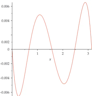
Example 4.3. In this example, let gx cosx and the interval be0, π; we consider its

approximating polynomial of degree 3:p3x. By Theorem3.1, we have

p3x 1−

3140π2_3π4₋₁₆₈₀

π5 x−

2160π2_π4₋₇₂₀

π6 x

2

14

60π2_π4₋₇₂₀

π7 x

3_,

3 2

1

x

−0.006

−0.004

−0.002 0 0.002 0.004 0.006

Figure 2:The residual errorcosx−p3xbetween cosxandp3xon0, π.

and the residual error cosx−p3 can be represented by Figure 2 . Obviously, the curve is

concussive; however, the residual error can reach 10−3.

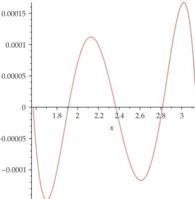
Example 4.4. Letgx sinxand the interval be π/2, π; we consider its approximating

polynomial of degree 4p4xby Theorem3.1. It is easy to verify

p4x 1−23π

5_8400π3_−127680π2_{−1532160π5806080}

π6

x−π

2

14

11π56000π3−110400π2−1209600π4700160

π7

x−π

2 2

− 56

7π5_4560π3_−95040π2_{−979200π3870720}

π8

x−π

2 3

336

π5_720π3_−16320π2_{−161280π645120}

π9

x−π

2 4

.

4.6

We plot the residual errorsinx−p4xin Figure3, where we find it can reach 10−4.

Acknowledgment

The work of the first author was supported in part by National Science Foundation for Young ScholarsGrant no. 60803076,61003186, the Natural Science Foundation of Zhejiang Province

3 2.8 2.6 2.4 2.2 2 1.8

x

−0.0001

−0.00005 0 0.00005 0.0001 0.00015

Figure 3:The residual errorsinx−p4xbetween sinxandp4xonπ/2, π.

References

1 D. S. Mitrinovi´c,Analytic Inequalities, Springer, New York, NY, USA, 1970.

2 R. P. Agarwal, Y.-H. Kim, and S. K. Sen, “A new refined Jordan’s inequality and its application,” Mathematical Inequalities & Applications, vol. 12, no. 2, pp. 255–264, 2009.

3 A. Baricz, “Some inequalities involving generalized Bessel functions,”´ Mathematical Inequalities & Applications, vol. 10, no. 4, pp. 827–842, 2007.

4 A. Baricz, “Jordan-type inequalities for generalized Bessel functions,”´ JIPAM. Journal of Inequalities in Pure and Applied Mathematics, vol. 9, no. 2, p. Article 39, 6, 2008.

5 A. Baricz, “Geometric properties of generalized Bessel functions,”´ Publicationes Mathematicae Debrecen, vol. 73, no. 1-2, pp. 155–178, 2008.

6 L. Debnath and C.-J. Zhao, “New strengthened Jordan’s inequality and its applications,” Applied Mathematics Letters, vol. 16, no. 4, pp. 557–560, 2003.

7 F. Y. Feng, “Jordan’s inequality,”Mathematics Magazine, vol. 69, no. 2, p. 126, 1996.

8 J.-L. Li, “An identity related to Jordan’s inequality,” International Journal of Mathematics and Mathematical Sciences, vol. 2006, Article ID 76782, 6 pages, 2006.

9 J. L. Li and Y. L. Li, “On the strengthened Jordan’s inequality,”Journal of Inequalities and Applications, vol. 2007, Article ID 74328, 9 pages, 2007.

10 A. McD. Mercer, U. Abel, and D. Caccia, “A sharpening of Jordan’s inequality,” The American Mathematical Monthly, vol. 93, no. 7, pp. 568–569, 1986.

11 D.-W. Niu, Z.-H. Huo, J. Cao, and F. Qi, “A general refinement of Jordan’s inequality and a refinement of L. Yang’s inequality,”Integral Transforms and Special Functions, vol. 19, no. 3-4, pp. 157–164, 2008.

12 A. Y. ¨Ozban, “A new refined form of Jordan’s inequality and its applications,”Applied Mathematics Letters, vol. 19, no. 2, pp. 155–160, 2006.

13 F. Qi and Q. D. Hao, “Refinements and sharpenings of Jordan’s and Kober’s inequality,”Mathematical Inequalities & Applications, vol. 8, no. 3, pp. 116–120, 1998.

14 F. Qi, L.-H. Cui, and S.-L. Xu, “Some inequalities constructed by Tchebysheff’s integral inequality,” Mathematical Inequalities & Applications, vol. 2, no. 4, pp. 517–528, 1999.

15 F. Qi, “Jordan’s Inequality: refinements, generalizations, applications and related problems,”RGMIA Research Report Collection, vol. 9, no. 3, article 12, 2006.

17 J. Sandor, “On the Concavity of sinx/x,”Octogon Mathematical Magazine, vol. 13, no. 1, pp. 406–407, 2005.

18 S. H. Wu, “On generalizations and refinements of Jordan type inequality,”RGMIA Research Report Collection, vol. 7, article 2, 2004.

19 W. S. H., “On Generalizations and Refinements of Jordan Type Inequality,”Octogon Mathematical Magazine, vol. 12, no. 1, pp. 267–272, 2004.

20 S. Wu and L. Debnath, “A new generalized and sharp version of Jordan’s inequality and its applications to the improvement of the Yang Le inequality,”Applied Mathematics Letters, vol. 19, no. 12, pp. 1378–1384, 2006.

21 S. H. Wu and L. Debnath, “A new generalized and sharp version of Jordan’s inequality and its applications to the improvement of the Yang Le inequality,II,”Applied Mathematics Letters, vol. 20, pp. 1414–1417, 2007.

22 S. Wu and L. Debnath, “Jordan-type inequalities for differentiable functions and their applications,” Applied Mathematics Letters, vol. 21, no. 8, pp. 803–809, 2008.

23 S.-H. Wu and H. M. Srivastava, “A further refinement of a Jordan type inequality and its application,” Applied Mathematics and Computation, vol. 197, no. 2, pp. 914–923, 2008.

24 S.-H. Wu, H. M. Srivastava, and L. Debnath, “Some refined families of Jordan-type inequalities and their applications,”Integral Transforms and Special Functions, vol. 19, no. 3-4, pp. 183–193, 2008.

25 C. J. Zhao, “Generalization and strengthen of Yang Le inequality,”Mathematics in Practice and Theory, vol. 30, no. 4, pp. 493–497, 2000Chinese.

26 L. Zhu, “Sharpening Jordan’s inequality and Yang Le inequality. II,”Applied Mathematics Letters, vol. 19, no. 9, pp. 990–994, 2006.

27 L. Zhu, “Sharpening of Jordan’s inequalities and its applications,” Mathematical Inequalities & Applications, vol. 9, no. 1, pp. 103–106, 2006.

28 L. Zhu, “A general refinement of Jordan-type inequality,”Computers & Mathematics with Applications, vol. 55, no. 11, pp. 2498–2505, 2008.

29 L. Zhu, “General forms of Jordan and Yang Le inequalities,”Applied Mathematics Letters, vol. 22, no. 2, pp. 236–241, 2009.

30 L. Zhu and J. Sun, “Six new Redheffer-type inequalities for circular and hyperbolic functions,” Computers & Mathematics with Applications, vol. 56, no. 2, pp. 522–529, 2008.