Proof for the Directivity of Circulation Intensity of Vector Field

2019 International Conference on Information Technology, Electrical and Electronic Engineering (ITEEE 2019) ISBN: 978-1-60595-606-0

Proof for the Directivity of Circulation Intensity of Vector Field

Hui-ting XU

1,*

, Ming-da XIONG

2

, Can-hui ZHANG

1

, Fang YANG

1

, Dan ZHAO

1

,

Jian-hong XIAO

1

and Long-min BU

1

1

State Grid Hunan Electric Power Limited Company Power Supply Service Center (Metrology Center), Hunan Province Key Laboratory of Intelligent Electrical Measurement and Application

Technology, China

2_{Yiyang Electric Power Company, China}

*Corresponding author

Keywords: Electromagnetic field, Curl, Circulation intensity, Vector analysis.

Abstract. At present, the introduction of curl is based on the directivity of circulation intensity, which means that circulation intensity under any given normal direction can be expressed as the scalar product between a vector (that is, the curl) and the unit vector in the normal direction. However, there is usually no enough explanation on the validity of the directivity characteristics. Beginning from the definition of circulation intensity, a detailed deduction procedure of the expression of circulation intensity was present under any normal direction by using a square integral path, and the validation of the directivity characteristics was verified. The work in this paper provides students with a feasible mathematical approach to understand the directivity characteristics, and can also be treated as a comprehensive exercise for vector analysis and field theory.

Introduction

As an extremely important basic concept in the Electromagnetic Field curriculum, curl has become one of the difficulties in the curriculum due to the abstract definition and complex mathematical definition. Generally, the logical order to introduce the curl in the “Electromagnetic Field” textbook is Circulation of Vector Field (contour integral)-Circulation Intensity (surface destiny of circulation)-Directivity of Circulation Intensity-Curl-Stokes Formula. As the very crucial knowledge point, the directivity of circulation intensity shows that circulation intensity can be expressed as the scalar product between a vector (the curl) and the unit vector in the normal direction of the integral path. Relationship between circulation intensity is similar to that between directional derivatives and gradient.

In the textbook of Electromagnetic Field, there are two primary methods to discuss the directivity characteristics of circulation intensity: 1) State without proof; 2) On the basis of Stokes Formula.

To be specific, in the first method, regarding the directivity characteristics as the known quantity, curl is introduced and its expression is solved without the proof of directivity. Considering the three micro rectangular loop as the study objects in the rectangular coordinate system, the circulation intensity of them can be worked out according to the definition. And the three circulation intensity can be treated as three components in the three coordinate axis directions, that is, curl is just the synthetic vector of the three components.

While, the second method transforms the circulation integral to the surface integral on the basis of Stokes Formula, which has been verified in the Higher Mathematics textbook without the concept of curl, and the expression and directivity characteristics are then solved.

For better understanding, the second method could be a nice choice. But it is in contrast with the logic order of Circulation-Circulation Intensity-Curl-the Stokes Formula, which has always been a preference in the Electromagnetic Field textbooks.

of circulation intensity, which is the best proof of the directivity characteristics, in any normal direction derived from the definition. It is in a sense similar to the process that directional derivatives in any direction be deduced from the definition formula of directional derivatives in scalar field, leading to find out the directivity characteristics of directional derivatives and introduce the concept of gradient.

In this paper, the expression of circulation intensity in any given normal directions is deduced from the definition in detail through the construction of a square integral path, and the concept of directivity characteristics and curl are then gained. The work in this paper can be treated as a comprehensive exercise for vector analysis and field theory.

Geometric Model e

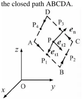
As shown in Fig.1, points A, B, C and D comprise a square, in which P is the center point and P1, P2, P3 and P4 are respectively the middle point of the 4 boundaries. en is a unit vector in the direction vertical to the plane in which the square is located, and en along with the directed closed path ABCDA conform to the Right-Hand Screw Rule. et1 and et2 are respectively the unit vector in the direction from P to P1 and the direction from P to P2. The following part of this paper is based on the assumption that the coordinate of point P is (x, y, z), and the edge length of square is a.

According to the definition, the circulation intensity of vector field F in the direction of en at point P can be expressed as follows:



2



n

0

fot lim

a  a



F (1)

[image:2.595.240.377.385.549.2]

where  is the circulation of F along the closed path ABCDA.

Figure 1. Schematic diagram of deduction of circulation intensity.

Since circulation intensity is the limit value of circulation/bounding area ratio when the closed path continuously shrinks into point P, the side lengtha is set to be a micro value. So, vector field in each side and the center can be treated as the same.  in Eq. 1 can then be written as:

 P1  P2  P3  P4

 F ABF BCF CDF DA (2)

First Order Approximately Expansion of Vector Function

In this part, the approximate values of vector field F at point P1, P2, P3 and P4 are derived by using first order Taylor expansion.

The component of F in P1 can be expressed as:

 

F

 

F

 

F

 

t1 t1 t1

cos , cos , cos

2  2  2 

a a a

x + y + z +

Then using first order Taylor expansion of multivariate function, the component in x axis of F(P1) can be expressed as:

                        

F a F a F a

F F

x y z

a

F F e

x x x

x 1 x t1 t1 t1

x x t1

P x, y, z cos cos cos

2 2 2

P 2

(4)

In the same way, components in axis y and z can be respectively written as:

 



   

 





F_y P₁ F_y P a2 F_x e_t1 (5)

 



   

 





F_z P₁ F_z P a 2 F_z e_t1 (6)

From (4) -(6) and (3), relationship between F(P1) and F(P) can be deduced as:

      





 

 



      _  _  _  _     

1 x t1 x y t1 y

z t1 z

P P 2

+

F F e e e e

e e

a F F

F (7)

In the same way, values of F at point P2, P3 and P4 can be expressed as follows:

      





 

 



      _   _  _  _      

2 x t2 x y t2 y

z t2 z

P P 2

+

F F e e e e

e e

a F F

F (8)

      





 

 



      _   _  _  _      

3 x t1 x y t1 y

z t1 z

P P 2

+

F F e e e e

e e

a F F

F (9)

      





 

 



      _  _  _  _     

4 x t2 x y t2 y

z t2 z

P P 2

+

F F e e e e

e e

a F F

F (10)

Calculation Formula of Circulation Intensity

After the text edit has been completed, the paper is ready for the template. Duplicate the template file by using the Save As command, and use the naming convention prescribed by your conference for the name of your paper. In this newly created file, highlight all of the contents and import your prepared text file. You are now ready to style your paper; use the scroll down window on the left of the MS Word Formatting toolbar.

In the square ABCD, 4 edge-vectors can be written as:

a t2,  a t1,  a t2, a t1

AB e BC e CD e DA e (11) Bring (7)-(11) back to (2), there is:













 

 

















   _   _  _  _       _   _  _  _       _   _  _  _ 2

x x t1 t2 x t2 t1

2

y y t1 t2 y t2 t1

2

z z t1 t2 z t2 t1

a F e F e

a F e F e

a F e F e

e e e

e e e

e e e

(12)











 







 

 

 





 











 







                                                        

x t1 t2 x t2 t1 x t2 t1 n x

y t1 t2 y t2 t1 y t2 t1 n y

z t1 t2 z t2 t1 z t2 t1 n z

F e F e F F

F e F e F F

F e F e F F

e e e e e

e e e e e

e e e e e

(13)

where et2 et1=-en and AB=-B A are as well involved. According to (12) and (13), there is:





 





  _   _ _   _    _   _ 2 2

x n x y n y

2

z n z

a F a F

a F

e e e e

e e

(14)

Applying the identity A (BC) =B (CA) to Eq. 14, three mixed products in the right side of Eq. 14 can be changed into:









 

 









    _   _  _  _     _   _  _  _     _   _   _  _

x n x n x x

y n y n y y

z n z n z z

F F

F F

F F

e e e e

e e e e

e e e e

(15)

Bring Eq. 15 back to Eq. 14, then simplify, there is:





 

 

  2  _        _

n x x y y z z

ae F e F e F e (16) The part in the bracket in (16) is defined as curl of vector field F:





 





  F F_x e_x F_y e_y F_z e_z (17) Curl in rectangular coordinate system can be reasonably expressed as:

y y

z x z x

x y z

x x             _  _ _  _ _  _            F F

F F F F

y z z y

F e e e (18)

Then, relationship between circulation intensity and curl can be deduced from Eq. 16 and Eq. 1 as follows:





  

n n

rot F e F (19) It is shown in Eq. 19 that, circulation intensity of vector field in some normal direction at one point is just a component of the curl in the mentioned normal direction. This is called directivity characteristics of circulation intensity.

Summary

In this paper, briefly based on the definition, the expression of circulation intensity in any normal direction is deduced with the help of square integral path, which has excellent symmetry. Directivity of circulation intensity could be apparently discovered on account of the mentioned expression, which provides with a more rigorous mathematic access for the introduction of curl, so as the explanation of relationship between circulation intensity and curl. Involving the first order approximate expansion and many vector identities, the derivation process in this paper can be also used as a comprehensive exercise for vector analysis and field theory.

References

[3] Zezhong Wang. Engineering Electromagnetics[M]. Beijing: Tsinghua University Press, 2011.

[4] Guangzheng Ni. Principles of engineering electromagnetic[M]. Beijing: Higher Education Press, 2009.

[5] Guru. B. S. Electromagnetic Field Theory Fundamentals[M]. Beijing: China Machine Press, 2002.

[6] Rugui Yang. Electromagnetic Field and Wave[M]. Xi'an: Xi'an Jiaotong University Press, 1989.

[7] Yinzhao Lei. Electromagnetic Field [M].Beijing: Higher Education Press, 2008.