O R I G I N A L A R T I C L E
Persistent threats to validity in single
‐
group interrupted time
series analysis with a cross over design
Ariel Linden DrPH
1,21
President, Linden Consulting Group, LLC, Ann Arbor, Michigan, USA
2
Research Scientist, Division of General Medicine, Medical School, University of Michigan, Ann Arbor, Michigan, USA
Correspondence
Ariel Linden, Linden Consulting Group, LLC, 1301 North Bay Drive, Ann Arbor, MI 48103, USA.
Email: [email protected]
Abstract
Rationale, aims and objectives
The basic single‐group interrupted time series analysis(ITSA) design has been shown to be susceptible to the most common threat to validity—history
—the possibility that some other event caused the observed effect in the time series. A single‐ group ITSA with a crossover design (in which the intervention is introduced and withdrawn 1
or more times) should be more robust. In this paper, we describe and empirically assess the
susceptibility of this design to bias from history.
Method
Time series data from 2 natural experiments (the effect of multiple repeals andreinstate-ments of Louisiana’s motorcycle helmet law on motorcycle fatalities and the association between the
implementation and withdrawal of Gorbachev’s antialcohol campaign with Russia’s mortality crisis)
are used to illustrate that history remains a threat to ITSA validity, even in a crossover design.
Results
Both empirical examples reveal that the single‐group ITSA with a crossover design may be biased because of history. In the case of motorcycle fatalities, helmet laws appearedeffective in reducing mortality (while repealing the law increased mortality), but when a control
group was added, it was shown that this trend was similar in both groups. In the case of
Gorbachev’s antialcohol campaign, only when contrasting the results against those of a control
group was the withdrawal of the campaign found to be the more likely culprit in explaining the
Russian mortality crisis than the collapse of the Soviet Union.
Conclusions
Even with a robust crossover design, single‐group ITSA models remainsusceptible to bias from history. Therefore, a comparable control group design should be
included, whenever possible.
K E Y W O R D S
causal inference, crossover design, interrupted time series analysis, quasi‐experimental
1
|I N T R O D U C T I O N
Single‐group interrupted time series analysis (ITSA) is a popular
evalu-ation strategy for observevalu-ational data in which a single unit is studied
(eg, an individual, a city, or a country), the dependent variable is a
seri-ally ordered time series, and multiple observations are captured in both
the pre‐and postintervention periods. The study design is called an
interrupted time series because the intervention is expected to
“interrupt”the level and/or trend of the time series, subsequent to
its introduction.1,2 It has been maintained that ITSA generally has
strong internal validity, primarily through its control overregression to the mean1–4and good external validity, particularly when the analysis occurs at the population level, or when the results can be generalized
to other units, treatments or settings.2,5
Recently, the validity of the basic single‐group ITSA design
(consisting of a preintervention phase and an intervention phase) has
been scrutinized. Linden6illustrated that this design can either fail to
identify the effects of external factors on the time series, resulting in
a false causal attribution, or conversely confuse the causal
interpreta-tion when a direcinterpreta-tionally correct change in the time series also occurs
before the intervention. In both cases, the inclusion of a comparable
control group clarifies causal effects.
[Correction added on 17 November 2016, after first online publication: The article’s title has been edited due to similarity with another of the author’s published article.]
DOI 10.1111/jep.12668
Shaddish et al2suggest adding design features such as the removal
of the treatment at a known time, or by extension, adding multiple
replications, to improve the validity of the single‐group ITSA design.
In essence, this is a single‐group version of the crossover design, in
which the intervention is introduced and withdrawn, 1 or more times.
The underlying premise is that it would be increasingly unlikely that
external events will affect the time series coincidentally with each
successive crossover, and thus, the results can be considered a causal
effect of the intervention if the time series changes accordingly.2
The purpose of the current paper is to offer a nontechnical
discus-sion of how, even with the addition of a crossover design, factors other
than the intervention may be mistaken for a treatment effect (or
with-drawal of treatment) when only a single group is being evaluated. By
way of example, it will be shown that the effects of external events
can only be identified and controlled for by utilizing a comparable control
group to serve as the counterfactual—a fundamental element of the
potential outcomes framework.7,8With the inclusion of a comparable
control group, factors other than the intervention that are responsible
for shifting the time series in each crossover phase will likely be observed
in both groups and thus, not mistaken for an effect of treatment or
withdrawal. Likewise, directionally correct changes that do occur in the
intervention group but not in the control group may be interpreted as
causal.9,10This problem is illustrated using data from 2 natural
experi-ments: the effect of multiple repeals and reinstatements of Louisiana’s
motorcycle helmet law on motorcycle fatalities and the association
between the implementation and the withdrawal of Gorbachev’s
antialcohol campaign and Russia’s mortality crisis in the early 1990s.
2
|T H R E A T S T O V A L I D I T Y I N T H E B A S I C
A N D C R O S S O V E R S I N G L E
‐
G R O U P I T S A
D E S I G N S
Although the basic single‐group ITSA design (consisting of a
preintervention and intervention phase) can control for many threats
to validity, the remaining threats that the design does not control for
are critical.1,2 Consequently, investigators typically add features to
the single‐group design, such as 1 or more treatment crossovers, with
the intent of mitigating the influence of these remaining biases.
Historyis the possibility that some event other than the interven-tion caused the observed effect in the time series,2and it is the
princi-pal threat to validity of any single‐group ITSA design. There are at least
2 scenarios where the effect of history may be overlooked or
misinterpreted. First, some factor may cause a directionally correct
change in the time series before the intervention. As such, any
addi-tional change in the time series subsequent to the introduction of
the intervention may be considered a continued or magnified effect
of that previous factor rather than a treatment effect.9Recently,
sen-sitivity tests adapted from the regression‐discontinuity literature11
have been applied to the ITSA design to identify these false treatment
effects.12In the second scenario, the change in the time series after
initiation of the intervention is immediate and drastic, and as such, it
is easy to ignore the possibility that some other factor may be the
cause. Even if there is an alternative explanation for the effect,
infor-mation may not always be available to identify those factors. Thus,
the investigator is likely to argue that the effect is causally related to
the intervention without further study.6
A crossover design is considered a more robust approach to
con-trol for history than the basic single‐group ITSA, by virtue of the fact
that there are more comparisons involved, making it less likely that
some external event will affect the time series repeatedly at each
crossover phase. For example, adding a specific time point when the
treatment is deliberately withdrawn allows the investigator to evaluate
change in the time series between 3 distinct phases (preintervention vs
intervention phase, intervention vs postintervention, and
preintervention vs postintervention). Conversely, in a simple ITSA
design, the intervention is considered ongoing, thereby limiting the
comparison to only the preintervention and intervention phase. If the
time series changes in the expected direction after each crossover,
then it may be harder to argue that the effect was caused by some
external event. In theory, as more crossovers are added to the study,
the threat of history should diminish accordingly. However, other
external events may in fact be causing changes in the time series
coin-cidentally with the initiation or withdrawal of the intervention,
regard-less of the number of crossovers. Only with the inclusion of a control
group for comparison, will the effect of external events on the time
series be identified.
Although history is the most common threat to validity, there are
at least 3 other threats to which ITSA is susceptible. Instrumentation,
or a change in how the time series is measured, is a threat to validity
that may erroneously appear as a treatment effect in both the basic
single‐group ITSA and crossover design.2 As an example, in health
management interventions, patients’health behaviors are sometimes
measured on different scales over time or a particular scale may be
altered.13,14As a result, the measurements will be both inconsistent
and unreliable. In general, although documentation should be obtained
indicating how and when the instrumentation changed, it may
never-theless be impossible to control for this bias in either a single‐group
ITSA or crossover design. However, with the inclusion of a comparable
control group, the change in instrumentation should affect both time
series equally, thereby nullifying its effect.
Selection may bias both the single‐group ITSA and crossover
design if the serial observations are cross‐sectional and the
character-istics (or composition) of the group under study are different in any 2
(or more) crossover phases of the study (selection is not a factor in
either a single‐group ITSA or crossover design where the same group,
or individual, undergoes surveillance over the duration of the study).
Selection may be controlled for by finding a control group that is
com-parable with the treatment group on preintervention characteristics (at
the very least, the groups should be comparable on the preintervention
level and trend of the outcome under study).9,10
Threats to statistical conclusion validity common to any study
design also apply to ITSA. These include low power, violated test
assumptions, and unreliability of measurement.2Although these issues
are important, their discussion is beyond the scope of this paper. The
reader is referred to Box and Tiao,15Glass et al,16McDowall et al,17
Crosbie,18 Gottman,19 Linden,9 Linden and Adams,10 McKnight
et al,20Simonton,21and Velicer and McDonald.22
In the following 2 empirical examples, we demonstrate the
In the first example, the data are analyzed as a single‐group ITSA
where the estimated effects substantiate the hypothesized effects.
Next, the time series for the intervention group is contrasted with that
of a control group to see if the treatment effects still stand. If the time
series for both groups are similar across all phases, then we have
dem-onstrated that the single‐group ITSA results are biased because of
his-tory (because events outside of the intervention are affecting the
control group as well). In the second example, the data are analyzed
as a single‐group ITSA where the estimated effects substantiate the
hypothesized effects. However, given that our focus in this example
is on the cause of the spike in the time series at the time of the
inter-vention’s withdrawal, the time series for the intervention group is
contrasted with that of several different control groups as sensitivity
analyses. History may be the source of bias if the time series spikes in
control groups where we hypothesize they should remain stable
(because an external event was causing a spike in both groups similarly).
3
|E X A M P L E 1 : T H E E F F E C T O F M U L T I P L E
R E P E A L S A N D R E I N S T A T E M E N T S O F
L O U I S I A N A
’
S M O T O R C Y C L E H E L M E T L A W
O N M O T O R C Y C L E D E A T H S
Louisiana first enacted a universal motorcycle helmet law in 1968.
Then in 1976, the law was partially repealed to require helmet use only
by riders younger than 18 years. In 1982, the universal helmet law was
reinstated. In 1999, the law was amended to require helmet use only
by motorcyclists younger than 18 years and riders older than 18 years
who did not have a minimum of $10,000 in medical insurance
cover-age. In 2004, the universal helmet law was again reinstated.23 This
unusual policy situation of multiple repeals/reinstatements (4 distinct
phases) of the law provides an excellent opportunity for testing the
validity of the single‐group ITSA crossover design to assess the effect
of the helmet law (and its repeal) on motorcycle fatalities.
For the current analysis, all motor vehicle fatality data for all states
were retrieved from the Fatal Accident Reporting System database for
the years 1975 to 2014 (which is all the data available in the system).24
Annual issues ofHighway Statisticsprovided motorcycle registration data for the periods of 1996 to 2001, and years between 1975 and
1996 were retrieved from the 1995 summary volume.25 Statistical
analyses were conducted using ITSA, a program written for Stata
14.1 (StataCorp., College Station, TX, USA) to conduct single‐group
and multiple‐group interrupted time series analyses.9,10When
compar-isons are made between times series on different scales or at different
levels of the same scale, the time series were ipsatively standardized26
to allow for comparisons on the same scale.
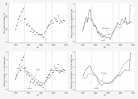
Figure 1A presents the raw motorcycle annual fatality counts in
Louisiana from 1975 to 2014. As shown, motorcycle deaths increased
from 1975 to 1982, the period in which the helmet law applied only to
riders younger than 18 years. Motorcycle deaths decreased annually
from 1982 to 1999, the period in which the universal helmet law
was reinstated. Motorcycle deaths increased annually from 1999 to
2004, the period in which the helmet law was once again applied only
[image:3.595.74.523.414.736.2]to riders younger than 18 years, and annual motorcycle deaths
appeared to stabilize (ie, the linear trend was flat) between 2004 and
2014, the period in which the universal helmet law was once again
reinstated.
As clearly illustrated in Figure 1A, the annual motorcycle fatalities
were directionally consistent with the expected effect. That is,
Louisiana’s multiple helmet law repeals were associated with increased
motorcycle fatalities, and the universal helmet law reinstatements
were associated with reduced or flat annual fatalities. In addition,
one could argue that most likely threats to validity2could be ruled
out. For example, there were a sufficient number of annual
observa-tions in each treatment phase (ie, repeal and reinstatement periods)
to rule out regression to the mean as a rival explanation.3,4Selection
bias may pose a threat to validity if the characteristics of those who
died in each treatment phase differed systematically from those who
died in the alternate treatment phase, with the most likely case being
made for differential fatality rates based on the age cutoff of 18 years.
However, an analysis by age‐group did not bear that out (data not
shown). History is a plausible threat to validity only if another event
or action had occurred concomitantly with the initiation of each
treat-ment phase. However, it is easy to dismiss the possibility that any
other factor could have caused the effect outside of the policy
changes, given such an immediate and dramatic effect that occurs
simultaneously with the initiation of each and every treatment phase.
However, Figure 1B casts doubt on the hypothesis that the
repeated repeals of the helmet law in Louisiana caused the increase
in motorcycle deaths. As shown, motorcycle registrations followed a
nearly identical historic pattern as motorcycle deaths, with the
excep-tion of the last few years of the data set, where a change in
methodol-ogy for estimating registered vehicles may have distorted the reporting
of registrations (a good example of instrumentation1,2). In light of these
data, one may revise the previous hypothesis to now consider that
motorcycle registrations hold the primary association with motorcycle
deaths in Louisiana, rather than the repeal and reinstatement of the
helmet law.
Figure 1C offers a complete rebuttal for any causal association
between Louisiana’s multiple helmet law repeals and reinstatements
and the change in motorcycle fatalities. Here, standardized motorcycle
fatalities in Louisiana are compared with those of all other States
(excluding Arkansas, Florida, Kentucky, Michigan, Pennsylvania, and
Texas—states that repealed their helmet laws during some point in
the same timeframe under study). As shown, the general behavior of
the time series in Louisiana is similar to that of all other states,
irrespective of the multiple repeals and reinstatements of the universal
helmet law in Louisiana.
Figure 1D illustrates standardized motorcycle registrations in
Louisiana and the control states over the entire observation period.
When paired with the corresponding motorcycle fatalities presented in
Figure 1C, the close relationship between registrations and fatalities
remains evident (until the mid‐2000s, when the change in
methodology for estimating registrations began to distort the
measurement of motorcycle registrations (for the details of the
meth-odological changes, see http://www‐fars.nhtsa.dot.gov/common/
FARS%20Encyclopedia%20VMT%20Changes.pdf).
In summary, despite improving the robustness of the single‐group
ITSA design by including multiple treatment crossovers (ie, repeal and
reinstatement), the effects of history still biased the results of the
eval-uation. Moreover, this bias was only revealed when Louisiana’s time
series was contrasted with that of the control states. The results of this
analysis suggest that motorcycle fatalities are not causally related to
the helmet law (ie, they do not decrease as a result of the law being
enacted/reinstated, and they do not increase as a result of the law
being repealed). However, given that motorcycle fatalities are so
closely associated to motorcycle registrations, an alternate hypothesis
may simply be that with more motorcycles on the road, there will be a
likewise increase in the number of fatalities.
4
|E X A M P L E 2 : T H E A S S O C I A T I O N
B E T W E E N G O R B A C H E V
’
S A N T I A L C O H O L
C A M P A I G N A N D R U S S I A
’
S M O R T A L I T Y
C R I S I S
In 1985, Mikhail Gorbachev initiated an antialcohol campaign
through-out the Soviet Union. The campaign was unprecedented in scale and
scope, and it operated through both supply‐side and demand‐side
channels, simultaneously raising the effective price of drinking and
subsidizing substitutes for alcohol consumption. At the height of the
campaign, official alcohol sales had fallen by as much as two thirds.
In practice, the campaign lasted beyond its official end in 1988, as
restarting state alcohol production took time, and alcohol prices
remained elevated.27
All‐cause mortality in the Soviet Union decreased during the
cam-paign years but rose precipitously between 1990 and 1994 (a period
that has been referred to as the“Russian mortality crisis”). Because this
episode also overlapped with Russia’s political and economic transition
to capitalism and democracy, the underlying cause of the mortality
crisis has been subject to considerable debate. However, Bhattacharya
et al27 provide a compelling argument that the mortality crisis was
mostly attributable to the coincident termination of the Gorbachev
antialcohol campaign rather than the political and economic transition.
For the present example, we reanalyze data from Bhattacharya
et al27in 2 ways. First, we conduct a single
‐group ITSA with a cross-over design to evaluate the effect of introducing and then withdrawing
the antialcohol campaign on mortality in Russia between the years
1960 and 2005. Next, we conduct separate multiple‐group ITSAs to
compare the mortality rates in Russia to those of 3 groups of countries
that would be expected to have a change in mortality rates
proportion-ate with their exposure to the antialcohol campaign and ethnic/
religious composition. The first group consists of former
Baltic/West-ern Soviet states that were exposed to the campaign and have a small
share of Muslims (Latvia, Lithuania, Estonia, Ukraine, Belarus, and
Mol-dova). The second group consists of former Soviet States that were
exposed to the campaign and have a large share of Muslims (Armenia,
Azerbaijan, Georgia, Uzbekistan, Kazakhstan, Krygyzstan, and
Turkmenistan), and the third group consists of non‐Soviet Eastern
European countries that were not exposed to the antialcohol campaign
at all but did undergo a similar political and economic transition (the
Czech Republic, the Slovak Republic, Hungary, and Poland).27
Considering the ethnic composition is important in this analysis
campaign would not be expected to significantly reduce mortality in
countries with large Muslim concentrations.27
In all analyses, the preintervention phase (ie, pre antialcohol
cam-paign) spans from 1960 to 1984; the intervention phase spans from
1985 to 1990; and the postintervention phase spans from 1991 to
2005 (3 distinct phases). As in the previous example, all statistical
anal-yses were conducted using ITSA,9,10 and for comparisons between
groups, the time series were ipsatively standardized to allow for
com-parisons between groups on the same scale.
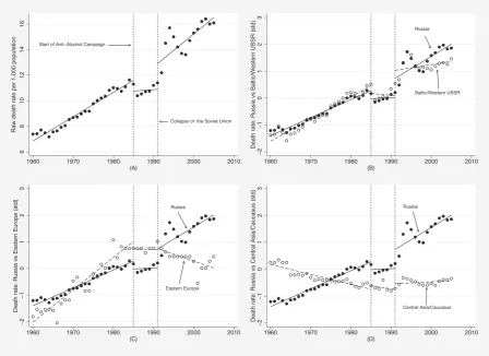
As illustrated in Figure 2, deaths per thousand increased linearly in
Russia from 1960 to 1985. There was a sharp drop in deaths
immedi-ately after the introduction of the antialcohol campaign in 1986, and
the level appears attenuated until 1991, at which point annual deaths
returned to the same level and trend of the time series before the
antialcohol campaign. The results from this single‐group ITSA indicate
that overall mortality rates in Russia decreased during the period of the
antialcohol campaign. However, this design does not provide an
unambiguous answer as to whether the decrease in mortality rates
was causally associated with the campaign, and whether the sharp rise
in mortality rates starting in 1991 was causally associated with the
withdrawal of the campaign.
Figure 2B shows the comparison of annual mortality rates in
Russia versus other former Soviet states that were also exposed to
the campaign and have low Muslim concentrations. As expected, these
states exhibited a trend in overall mortality similar to that of Russia,
thereby confirming that the antialcohol campaign was equally effective
in other states exposed to intervention with a similar demographic
composition.
Figure 2C shows the comparison of annual mortality rates in
Russia versus other non‐Soviet Eastern European countries that were
not exposed to the antialcohol campaign but did undergo a political
and economic transition as well. As illustrated, mortality rates in non‐
Soviet countries rose over time before the campaign (between 1960
and 1985) then flattened during the period of the campaign, but in
contrast to Russia, it declined after 1991. Although this may call into
question the causal relationship between campaign and mortality
(given that both Russia and non‐Soviet Eastern bloc countries
experi-enced a flat trend in mortality during the campaign years), it does
sug-gest that withdrawal of the campaign was more causally associated
with the Russian mortality crisis than the political and economic
transitions (given that the transition occurred across all these countries
contemporaneously).
Figure 2D shows the comparison of annual mortality rates in
Russia versus those of former Soviet states with higher concentrations
of Muslims. As hypothesized, the trend in mortality rates of the Central
Asia/Caucasus countries followed a completely different pattern than
that of Russia. In these former Soviet states, mortality rates declined
from 1960 to 1990 and then appeared to stabilize over the
remaining duration of the study. If the Russian mortality crisis was
entirely due to the political and economic transition and not
withdrawal of the antialcohol campaign, we would expect to see a
[image:5.595.74.523.400.726.2]comparable increase in mortality in this set of former Soviet states
that also experienced the transition but were not sensitive to the
antialcohol policy.
In summary, this example again highlights the effect of history
in complicating the interpretation of ITSA results—even when
utilizing a crossover design. Only when contrasting the results
against those of a control group (or in this case, against different
sets of control groups) was the treatment effect of Gorbachev’s
antialcohol campaign substantiated, and relatedly, the withdrawal
of the campaign was found to be the more likely culprit in
explaining the Russian mortality crisis than Russia’s transition to
capitalism and democracy.
5
|D I S C U S S I O N
The 2 examples presented in this paper suggest that the single‐group
ITSA crossover design is just as vulnerable to the effects of history
as the basic single‐group ITSA design.6In the first example, a seemingly
unquestionable treatment effect (and withdrawal effect) across
multi-ple crossovers was reversed when contrasted with a comparable
con-trol group. In the second example, a negative change in the time series
after withdrawal of the intervention was attributed to an external
event, and only when compared with a control group did the
with-drawal of the intervention receive correct attribution for that effect.
In short, even with the addition of 1 or more crossovers, a single‐group
ITSA remains susceptible to threats to validity that limit the ability to
draw causal inferences about the effects of the intervention.
As demonstrated in the present examples (in addition to those
presented in Linden6), using a control group to serve as the
counterfac-tual is the most robust approach for assessing treatment effects. Only
when contrasted with a comparable control group can the effect of the
intervention (or withdrawal of the intervention) be isolated from other
rival factors. Moreover, other anomalies observed in the time series
(eg, changes in instrumentation, selection bias) can alert the
investiga-tor to other potential sources of confounding.
When multiple nontreated units are available, investigators can
choose from at least 3 different matching methods suitable for time
series data. This includes the matching process implemented in the
present examples (ie, finding nontreated units that are nonstatistically
different from the treated unit on preintervention levels and trend of
the outcome variable),9a synthetic controls approach28or propensity
score‐based weighting10 (which can also be extended to situations
in which multiple treated units are available)29 and for censored
data.30,31Investigators should also consider the use of an
instrumen-tal variables strategy in cases where some of the right‐hand side
covariates are endogenous.32–34 Most statistical software packages
have commands designed to implement these approaches (such as
XTIVREG in Stata).
Finally, although this paper has illustrated that the crossover
design does not ensure improved validity when implemented in a
sin-gle‐group study, the crossover design can further enhance the
robust-ness of an ITSA study that includes a comparable control group to
serve as the counterfactual. In such a study, the groups switch their
treatment assignment at a given time point (ie, the treatment group
switches to control and the control switches to treatment) and the
outcomes change in accordance with the exposure to the
intervention. Although clearly difficult to implement in practice, the
design, when properly executed, may possibly be considered as good
as randomized (see Barlow et al35and Biglan et al36for other ITSA
design alternatives to improve causal inference over the basic
single‐group design).
In summary, this paper illustrated that history—the foremost
threat to validity in the basic single‐group ITSA design—persists even
when adding 1 or more treatment crossovers to the study. Absent a
comparable control group as a contrast, there is simply no assurance
that the effect of external factors have been identified and controlled
for, regardless of whether the time series follow the expected pattern
after each crossover. Thus, even when using a single‐group ITSA
cross-over design, the results should be considered preliminary—and
interpreted with caution—until a more robust study design can be
implemented. Given the popularity and widespread use of single‐group
ITSA designs, it is important for investigators to be cognizant of their
limitations and to strive to add a comparable control group to maximize
validity and improve causal inference.
A C K N O W L E D G M E N T S
The author thanks Grant Miller for providing the data used in the
second example of this paper. He also thanks Julia Adler‐Milstein for
reviewing the manuscript and for providing many helpful comments.
R E F E R E N C E S
1. Campbell DT, Stanley JC.Experimental and Quasi‐Experimental Designs for Research. Chicago, IL: Rand McNally; 1966.
2. Shadish WR, Cook TD, Campbell DT. Experimental and Quasi‐ Experimental Designs for Generalized Causal Inference. Boston: Houghton Mifflin; 2002.
3. Linden A. Estimating the effect of regression to the mean in health management programs.Dis Manag Health Out. 2007;15:7–12. 4. Linden A. Assessing regression to the mean effects in health care
initiatives.BMC Med Res Methodol. 2013;13:1–7.
5. Linden A, Adams J, Roberts N. The generalizability of disease management program results: getting from here to there.Manag Care Interface. 2004;17:38–45.
6. Linden A. Challenges to validity in single‐group interrupted time series analysis.J Eval Clin Pract. 2017;23:413–418.
7. Rubin DB. Estimating causal effects of treatments in randomized and nonrandomized studies.J Educ Psychol. 1974;66:688–701.
8. Rubin DB. Causal inference using potential outcomes: design, modeling, decisions.J Am Stat Assoc. 2005;100:322–331.
9. Linden A. Conducting interrupted time‐series analysis for single‐and multiple‐group comparisons.Stata J. 2015;15:480–500.
10. Linden A, Adams JL. Applying a propensity‐score based weighting model to interrupted time series data: improving causal inference in program evaluation.J Eval Clin Pract. 2011;17:1231–1238.
11. Linden A, Adams JL. Combining the regression‐discontinuity design and propensity‐score based weighting to improve causal inference in program evaluation.J Eval Clin Pract. 2012;18(2):317–325.
12. Linden A, Yarnold PR. Using machine learning to identify structural breaks in single‐group interrupted time series designs.J Eval Clin Pract. 2016;22:851–855.
13. Linden A, Roberts N. Disease management interventions: what’s in the black box?Dis Manag. 2004;7(4):275–291.
15. Box GEP, Tiao GC. Intervention analysis with applications to economic and environmental problems.J Am Stat Assoc. 1975;70:70–79. 16. Glass GV, Willson VL, Gottman JM.Design and Analysis of Time‐Series
Experiments. Boulder: University of Colorado Press; 1975.
17. McDowall D, McCleary R, Meidinger EE, Hay RA. Interrupted Time Series Analysis. Newbury Park, CA: Sage Publications, Inc; 1980. 18. Crosbie J. (1993) Interrupted time‐series analysis with brief single‐
subject data. J Consult Clin Psychol. 1993;61:966–974.
19. Gottman JM. Time‐series analysis. A Comprehensive Introduction for Social Scientists. New York: Cambridge University Press; 1981.
20. McKnight S, McKean JW, Huitema BE. A double bootstrap method to analyze linear models with autoregressive error terms.Psychol Methods. 2000;5:87–101.
21. Simonton DK. Cross‐sectional time‐series experiments: some suggested statistical analyses.Psychol Bull. 1977;84:489–502. 22. Velicer WF, McDonald RP. (1991) Cross‐sectional time series designs: a
general transformation approach. Multivariate Behav Res. 1991;26:247–254.
23. Chaudhary GH, Neil K, Solomon MG, Preusser DF, Cosgrove LA. Eval-uation of the Reinstatement of the Helmet Law in Louisiana. National Highway Traffic Safety Administration. 2008. Available at: www. nhtsa.gov/DOT/NHTSA/Traffic%20Injury%20Control/Articles/Asso-ciated%20Files/810956.pdf. Accessed September 7, 2016.
24. U.S. Department of Transportation, National Highway Traffic Safety Administration, National Center for Statistics and Analysis. Fatality Analysis Reporting System (FARS). Available at: ftp://ftp.nhtsa.dot. gov/fars/. Accessed September 7, 2016.
25. U.S. Department of Transportation, Federal Highway Administration. Highway Statistics (Multiple Years). Available at: http://www.fhwa. dot.gov/policyinformation/statistics.cfm. Accessed on September 7, 2016.
26. Yarnold PR, Linden A. Using machine learning to model dose‐response relationships via ODA: eliminating response variable baseline variation by ipsative standardization.Optimal Data Analysis. 2016;5:41–52.
27. Bhattacharya J, Gathmann C, Miller G. The Gorbachev anti‐alcohol campaign and Russia’s mortality crisis. Am Econ J Appl Econ. 2013;5:232–260.
28. Abadie A, Diamond A, Hainmueller J. Synthetic control methods for comparative case studies: estimating the effect of California’s tobacco control program.J Am Stat Assoc. 2010;105:493–505.
29. Linden A, Adams JL. Evaluating health management programmes over time. Application of propensity score‐based weighting to longitudinal data.J Eval Clin Pract. 2010;16:180–185.
30. Robins JM, Hernán MA, Brumback B. Marginal structural models and causal inference in epidemiology.Epidemiology. 2000;11:550–560. 31. Linden A, Adams J, Roberts N. Evaluating disease management
program effectiveness: an introduction to survival analysis.Dis Manag. 2004;7:180–190.
32. Linden A, Adams J. Evaluating disease management program effectiveness: an introduction to instrumental variables. J Eval Clin Pract. 2006;12(2):148–154.
33. Baltagi BH.Econometric Analysis of Panel Data. 4th ed. New York: Wiley; 2008.
34. Becketti S.Introduction to Time Series Using Stata. College Station, TX: Stata Press; 2013.
35. Barlow DH, Hayes SC, Nelson RO.The Scientist Practitioner: Research and Accountability in Clinical and Educational Settings. New York: Pergamon Press; 1984.
36. Biglan A, Ary D, Wagenaar AC. The value of interrupted time‐series experiments for community intervention research. Prev Sci. 2000;1:31–49.
How to cite this article: Linden A. Persistent threats to
valid-ity in single‐group interrupted time series analysis with a cross