An Ef
fi
cient Method for Selecting the
Optimal Structure of a Fuzzy Neural
Network Architecture
Bojan Novak
University of Maribor, Faculty of Electrical Engineering and Computer Science, Maribor, Slovenia
The fusion of artificial neural networks with soft com-puting enables to construct learning machines that are superior compared to classical artificial neural networks, because knowledge can be extracted and explained in the form of simple rules. An efficient method for selecting the optimal structure of a fuzzy neural network archi-tecture is developed. The Vapnik Chervonenkis (VC)
dimension is introduced as a measure of the capacity of the learning machine. A prediction of the expected error on the yet unseen examples is estimated with the help of the VC dimension. The structural risk minimization principle is introduced for constructing the optimal ar-chitecture with the lowest expected error for the small data sets. A comparison between fuzzy neural network and the neural network ARX model is presented.
Keywords: soft computing, learning theory, neural net-works
1. Introduction
In 1958, Rosenblatt developed a biologically in-spired learning machine simulated on the com-puter. Its name was Perceptron and it was able to solve a simple pattern recognition task and was able to generalize. A whole new field of learn-ing machines appeared with the common name artificial neural networks. An effective method to describe the general principle of inductive inference in different machines was developed by Vapnik and Chervonenkis at the end of the 1960s. It is known as the empirical risk min-imization (ERM) principle. At the beginning
the theory was developed for pattern recogni-tion but was later extended for funcrecogni-tion approx-imation, regression estapprox-imation, estimating the values of function at given points, estimating
the function on the basis of indirect measure-ments and similar. The necessary and sufficient conditions for consistency of the ERM principle were first developed for the indicator functions
(having 0,1 values). During the learning
pro-cess the empirical risk is minimized on these indicator functions. This is the first necessary step. Second is to define theoretically as accu-rate as possible the bounds on the probability of the test error on yet unseen examples for the function minimizing the empirical risk.
The application of the ERM principle generates the best possible solution with the increasing number of examples only in cases where the uniform law of large numbers applies. Uniform law of large numbers is defined: the frequency of an event converges to the probability of this event with the increasing number of observa-tions over all sets of events defined by indicator functions implemented by the learning machine. In the late 1960s Vapnik and Chervonenkis de-fined the conditions where the uniform law of large numbers held for a given set of events and the bounds on the nonasymptotic rate of uniform convergence. They introduced a capacity con-cept for the set of indicator functions – the VC dimension, which characterizes the variability of the set of indicator functions. The maximum number of different binary(values 0 or 1)
parti-tioning ofksamples is 2k. The growth function is defined as
G(k) kln 2: (1.1)
to have fast convergence is
lim
k!1
G(k)
k =0: (1.2)
If, for an indicator function, the expression(1.1)
is valid for anyk, then such a function is able to split any sample of arbitrary size, in all pos-sible ways, or it is able to fit any data set with zero error. Later on, the well-known problem of over-fitting arises. A requirement for an indica-tor function is that after some finite value ofkits growth is less thankln 2. This values is the VC dimension – h (VC = Vapnik Chervonenkis) Vapnik et al. (1996), Vapnik (1998)]. Then
the growth function is logarithmically bounded
GΛ(k)= (
kln 2 ifk h h
1+ln
k h
ifk >h
(1.3)
where GΛ(k) is a growth function of a set of
indicator functionsQ(xα),α 2 Λ andα
rep-resent a capacity ability and Q(xα) presents
convex penalty term. For example, it could be the order of the polynomial chosen from the fi-nite set of ordersΛ. In the case of real functions the VC dimension is bounded.
2. Algorithm Description
For the givenkobservations each consisting of a pair: xi, yi, where xi 2 R
n
i = 1:::k is
the input vector and yi is the associated
out-put. The learning machine is actually building up a mapping ability x ! f(xα) where the
functions f(xα)themselves are labeled by
ad-justable parametersα. The expectation of the test error for the trained machine is
Rf]= Z
1
2L(y; f(xα)dP(xy)): (2.1)
Rf]is the risk functional. Pis the probability
and L presents loss function (could be in the
form such as that in the(2.2)). The mean error
rate measured on the finite number of observa-tions is the “empirical risk”
Remp(α)=
1
k
k X
i=1
(y; f(xiα))
2
: (2.2)
Remp(α) is fixed for a particular choice of α
and for a particular training setfxiyigand the
probability is not included in the equation. The expression(yi;f(xiα))
2is the loss function.
The empirical risk minimization does not im-ply a small error on the test set if the num-ber of examples in the training data set is lim-ited. The structural risk minimization is one of the new techniques for handling efficiently a limited amount of data. For a probability 1;ηη : 0 η 1 the bound holds that
depends on the parameterΦwhich is defined as
Φ
h k
log(η)
k = v u u th
log2k
h +1 ;log η 4 k R(α)
Remp(α)
1;Φ
h k
log(η)
k
: (2.3)
R(α)is the actual error on the previously unseen
examples. The parameterhis the VC dimension
Sch¨olkopf et al. (1995), Vapnik et al. (1996),
Vapnik(1998)]. It describes the capacity of a
set of functions implemented on the learning machine.
According to the eq. (2.3) risk could be
con-trolled by two quantities: Remp(α) and
h(ff(xα) : α 2 ksubg), where ksub is some
subset of the index set k. The empirical risk
Rempdepends on the choice of the optimal
func-tion(α)applied in the learning machine. The
VC dimension h depends on the set of func-tionsff(xα): α 2ksubg. The parameterhis
controlled by introducing the structure of nested subsetsSn:=ff(xα):α 2kng,
S1S2 S3:::Sn::: (2.4)
with the adequate VC dimensions satisfying
h1 h2 ::::::hn ::::::
The structural minimization principle chooses the function f(xα
) in the subset ff(xα) :
α 2 kng with the minimal right hand side of
the eq. (2.3). The guaranteed risk bound is
minimal. In the case of prediction, a nonlinear function f(α) has to be constructed that gives
minimal error on the test data (data not from
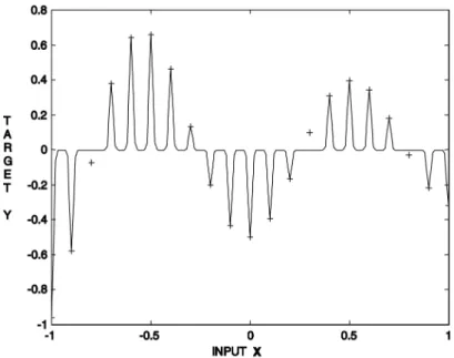
Fig. 2.1Improper complexity – overfit.
procedure. Because of the simplicity the linear case will be explained first
f(x) =w Tx
+b: (2.5)
The optimal parameter w and b could be cal-culated through empirical error minimization
(2.2).
Complex functions can easy generate zero train-ing errors. In the fig. 2.1 there is a simple exam-ple of regression function with high comexam-plex- complex-ity. The function goes(almost)exactly through
learning points(marked with anx), but for other
points between them, it produces meaningless results. This effect is known also as overfit. In practice, only limited amounts of data are available. That implies that any regression model will be inaccurate – biased. More com-plex functions require exponentially more data. This means that building regression model solely on the empirical risk minimization defined in
(2.2)is inadequate. It has to be expanded by a
term that forces optimal model by lowest possi-ble complexity. This is achieved by regularized riskRreg
Rreg =Remp+λkwk
2
2: (2.6)
The regularization parameterλ regulates influ-ence of the penalization term. In the case of lin-ear regression we would like to find the function
(represented by coefficientsw)with the
small-est steepness among the functions that minimize
(2.2). There is always some imprecision in the
data set – noise. Therefore some small toler-ance in errorsε should be allowed and problem
(2.6)can be solved as optimization problem
min1 2kwk
2
2 (2.7)
with respect to the constraints
y1 =w Tx
i;b ε
wTxi+b;yi ε:
In the formulation(2.7)we rely on the
assump-tion that the convex optimizaassump-tion problem is feasible. Sometimes this may not be the case and slack variablesξ are introduced to deal with otherwise infeasible constraints of the optimiza-tion problem(2.7)
min1 2kwk
2 2+C
k X
i=1
(ξi+ξ
i ) (2.8)
with respect to constraints
y1;w Tx
i;b ε +ξi
wTxi+b;yi ε +ξ
i
ξiξ i 0:
The constantC > 0 regulates the trade off
which deviations larger thanεare tolerated. The
ξ insensitive loss function is defined
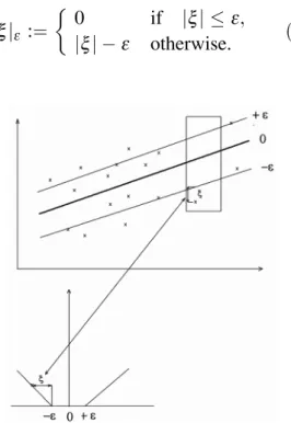
jξjε :=
0 if jξj ε
jξj;ε otherwise.
(2.9)
Fig. 2.2ξinsensitive loss function.
Graphically the ε insensitive loss is presented in fig. 2.2. Above is inputxon the abscise and
y = f(x) on the ordinate. Below is ε on the
abscise and penalty value on the ordinate. Only the points outside +ε and ;ε area contribute
to the rise of the value in (2.8). For example,
the point x marked withζi, that is outside ε
region(fig. 2.2)above, is linearly penalized by
the amount shown below. All points insideε
region are not penalized.
The problem(2.8)can be handled more easily as
the dual quadratic program. A Lagrange tion is constructed from both objective func-tion(it will be called primal objective function)
and the corresponding constraints by introduc-ing dual set of variables. It can be shown that this function has a saddle point with respect to the primal and dual variables at the optimal solutionMangasarian (1969)]. The Lagrange
function has the following form
L:=
1 2kwk
2 2+C
k X
i=1
(ξi+ξ i )
; k X
i=1
α1(ε +ξi;yi+w Tx
i+b)
; k X
i=1
α i(ε +ξ
i +yi;w Tx
i;b)
; k X
i=1
(ηiξi+η iξ
i): (2.10)
The dual variables in(2.10)have to satisfy
con-straints αiα iηiη
i 0. From the saddle
point the condition follows
@bL= k X
i=1 (α
i ;αi)=0 (2.11)
@wL =w; k X
i=1 (α
i ;α1)xi =0 (2.12)
@ξ ( )L
=C;α () i ;η
()
i =0: (2.13)
Substituting(2.11),(2.12)and(2.13)into(2.10)
yields dual optimization problemVapnik 1998]
where now the maximum is searched
max;
1 2
k X i j=1
(αi;α
i)(αj;α j)xixj
;ε k X i j=1
(αi+α i)+
k X
i=1
yi(αi;α i) (2.14)
with respect to the constraints
k X
i=1
(αi;α i)=0
αiα
i 20C]:
Dual variables ηiη
i are eliminated through
condition(2.13)Vapnik 1998]. As values can
be above ε region or below ;ε region,
vari-ables are separated intoαiηiξ andα iη
iξ
.
From(2.12)wcan be expressed
w=
k X
i=1 (α
i ;αi)xi
and(2.5)can be expressed in the form of
f(x)= SV X
i=1 (α
The form(2.15)is the support vector expansion
of the linear regression.
The coefficientbcan be computed by exploiting Karush-Khun-Tucker conditionsKarush(1939)], Kuhn et al.(1951)]. These state that at the
opti-mal solution the product between dual variables and constraints has to vanish. In our case this means
αi(ε +ξi;yi+wxi+b)=0
α i(ε +ξ
i +yi;wxi;b)=0
(2.16)
(C;αi)ξi=0 (C;α
i)ξ
i =0:
(2.17)
From(2.16)it follows that only samples(xiyi)
with corresponding α()
i = C lie outside ε;
insensitive tube around f. Situationαiα i = 0
means that both variables cannot be nonzero at the same time. This would require nonzero slack variables in both directions. For α()
i 2 0C] we have ξ
()
i = 0 and the second factor
in(2.16)must vanish. It follows
b=yi;wxi;ε =0 for αi2(0C)
b=yi;wxi+ε =0 for α
i 2(0C): (2.18)
From (2.16) it follows that only for jf(xi) ;
yijεthe Lagrange multipliers may be nonzero.
For all samples inside theε;tubeαiα i
van-ish. For jf(xi) ; yij < ε second factor is
nonzero. Because of Karush-Khun-Tucker con-ditionsαiα
i has to be zero. Therefore, we have
sparse expansions ofwin terms ofxi. In other
words, we do not need allxito describew.
Ex-amples with the vanishing coefficient are called support vectors.
The regression algorithm is made nonlinear by applying mapΦ:X!Fand then the standard
regression algorithm. An example of such map isΦ:R
2
!R
3
Φ(x1x2)=(x
2 1
p
2x1x2x
2
2): (2.19)
Where subscripts in this case refer to the com-ponents of x 2 R
2. For higher order maps
analytical expressions become impossible. The work around is implicit mapping via kernels
K(xx T
) := Φ(x) Φ(x T
) instead of using
Φ(x) explicitly ( is dot product). Now we
can rewrite(2.14)as follows
max;
1 2
k X i j=1
(αi;α
i)(αj;α
j)K(xixj)
;ε k X i j=1
(αi+α i)+
k X
i=1
yi(αi;α i) (2. 20)
with respect to the constraints
k X
i=1
(αi+α i)=0
αiα
i 20C]:
The expansion ofw
w=
k X
i=1 (α
i ;αi)Φ(xi)
and functionf in(2.15)can be expressed in the
form of
f(x) = k X
i=1 (α
i ;i)K(xix)+b: (2.21)
Optimization problem now corresponds to find-ing the flattest function in the feature space and not in the original input space.
The fusion of ANN with soft computing enables construction of a new learning machine that is superior compared to classical ANN, because knowledge can be extracted and explained in the form of simple rules Zadeh (1997)]. The
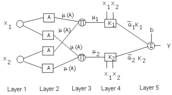
following new support vector FANN architec-ture can be defined as presented in the fig. 2.3. Layer 1 calculates membership values. Layer 2 performs T norm operator (multiplication).
Layer 3 derives the product of each rule’s out-put. Layer 4 performs the kernel Gaussian ra-dial basis operation (2.22). Layer 5 sums its
inputs as the overall output whereα =α i ;αi.
In the model presented here, the membership functions are in the form of Gaussian functions:
K(xxi)=exp
;
(x;xi)
2
2σ2
: (2.22)
Fig. 2.3Support vector FANN architecture.
so application of clustering methodsBezdek et
al. (1987), Chiu (1994), Yager et al. (1994)]
is unnecessary. The basis widthσ of(2.22) is
selected by structural minimization principles
(2.3)and(2.4). The output from the FANN is
f(x)= SV X
i=1 (α
i ;αi)K(xix)+b (2.23)
whereSV is the number of support vectors.
3. Case Study
An example of application of the above theory is shown with regard to the daily electrical energy consumption Srinivasan et al. (1995)]. The
data set that consists of meteorological data(xi)
and daily energy consumption(yi). The data set
is preprocessed to present only days from Mon-day to FriMon-day, without holiMon-days or any other outliers. The identification task is a multiple in-put single outin-put type problem. The outin-put was the prediction of daily energy consumption. The idea applied here is to use only a part of the data set(a window)due to the nature of the
problem. Therefore, only local data(around the
date of prediction)from each year is taken as the
learning set. This technique cannot be applied using the standard time series methods, because
the data set in this case is too small. The struc-tural risk minimization principle was applied to minimize expected risk (2.4). For each
pre-dicted point in fig. 3.1 optimization problem
(2,20)in feature space is solved. Prediction is
calculated with(2.23).
For comparison purpose two different appro-aches for nonlinear system identification were applied to the described problem. The first method is extension of the classical identifica-tion model ARX, where implementaidentifica-tion is done with the help of neural networks (NNARX).
This model does not include feedback and does not pose the stability problems, which can occur in recurrent networks such as NNARMAX and other similar techniques. The second method is a window based fuzzy identification method described above.
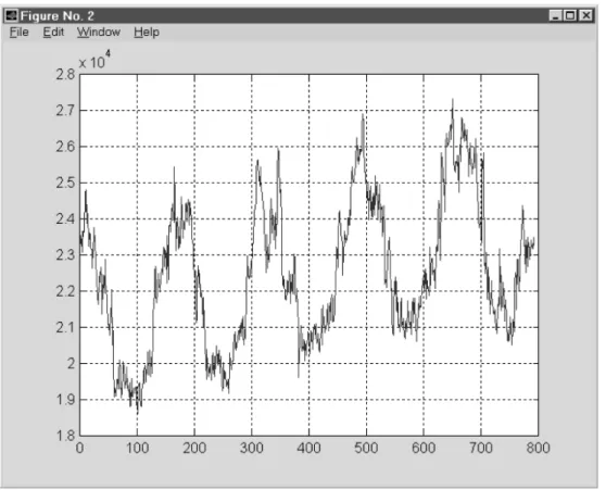
The task is to identify the shape of an energy consumption curve and afterwards make pre-dictions(fig. 3.1). The database consists of the
data for five years, where the last 30 days are removed for testing a prediction error.
In the system identification theory, different models exist for nonlinear identification. In our approach, we have chosen the ARX model
Ljung(1997)], modeled by regressor vector: Φ(t)=y(t;1):::y(t;na)u(t;nk):::
u(t;nb;nk+1)]
T
Fig. 3.1Daily energy consumption curve for the work days.
y(t)=the output at the sampling timet
u(t)=the input at the sampling timet
na=the number of the past outputs
nb=the number of the past inputs
nk=the time delay(nk =1 usually)
and the predictor:
_
y(tΘ)=(tjt;1Θ)=g(ϕ(t)Θ) (3.2)
_
y (tΘ)=is the predicted output
g(ϕ(t)Θ)=is the function realized by the
ar-tificial neural network(ANN).
Θ=is a vector of weights of the ANN.
In our case study, the ANN is a multilayer per-ceptron(MLP)with one hidden layer. For the
given training set:
ZN =fu(t)y(t)]jt=1:::Ng (3.3)
training the MLP presents a mapping from the set of the training data to the set of possible weights such that
ZN ! _
Θ : (3.4)
In addition, the network will produce output, which is given by
_
y(tΘ) y(tΘ) (3.5)
where the predicted value will be as close as possible to the true datay.
The prediction-error-approach is used to mini-mize the square of error
minVN(ΘZ N
)=
1
N
N X
i=1
(y(t); _
y(tjΘ))
2
:
(3.6)
Minimization is done with the Levenberg-Mar-quardt method Nørgaard (1997)]. However,
this is not an easy task because of the following problems
1) selecting a proper model structure(
complex-ity),
2) multiple minima exist in the error surface
Performances of the FANN versus the NNARX are presented for the case of a daily electrical energy consumption prediction. The learning data set consists of meteorological data and the energy from the previous days. The data are pre-processed to present only the days from Monday to Friday, without holidays or any other outliers. The trend is obvious in fig. 3.1 and to make the curve stationary, it was removed before the learning phase.
Due to the nature of the problem, in the case of training the FANN only a part of the data set(a
window around the date of the prediction)was
used. This technique cannot be applied using the NNARX model, because the data set in this case is too small. For the NNARX the classical time series approach was used with the daily en-ergy consumption from the previous days and meteorological data for the same days and pre-dicted values(from the weather forecast)for the
day of prediction.
The FANN structure enables extracting the rules in the “if – then” form from the positions and the width(σ)of the membership functions for
the each input. By applying these rules the FANN can explain each particular prediction it has made. Standard ANNs are not able to explain their conclusions. Only limited infor-mation about their conclusion – making process can be devised from Hinton diagrams.
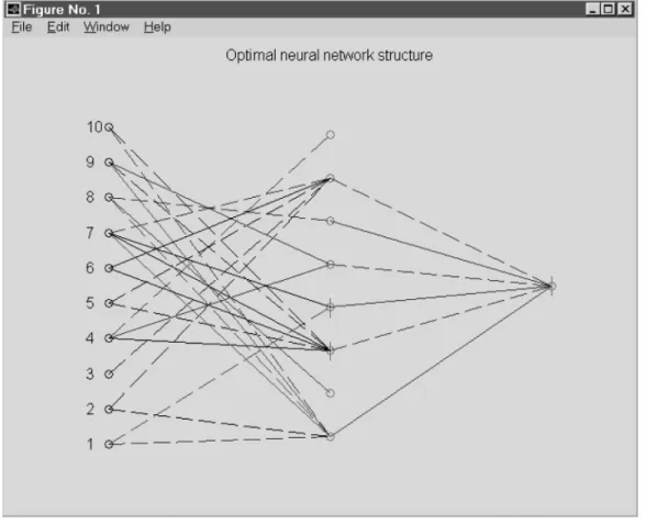
To achieve the best prediction accuracy for the NNARX model, optimal pruning method was applied. The result of optimization is given in the fig. 3.2, where unnecessary nodes were pruned. The pruning procedure used in this study is based on the modified method of Hansen and Pedersen Hansen et al. (1994)].
This technique stems from the so-called opti-mal brain surgeon method developed by Has-sibi and StorkHassibi et al.(1993)]. The
Neu-ral Network Based System Identification Tool-box developed by Magnus NørgaardNørgaard
(1997)] was applied for modeling and
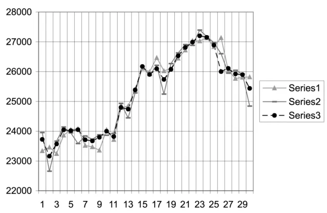
opti-mizing NNARX. In fig. 3.3 daily energy con-sumption predictions are presented, made by the FANN and the NNARX for the 30 days time period. The FANN window based method achieved about 10% better prediction accuracy.
Fig. 3.3Comparison of the results, 1=NNARX, 2=actual, 3=FANN.
4. Conclusion
The fusion of artificial neural networks with soft computing enables to construct learning ma-chines that are superior compared to classical artificial neural networks because knowledge can be extracted and explained in the form of simple rules. An efficient method for selecting the optimal structure of a fuzzy neural network architecture is developed and a new fuzzy neural architecture is introduced. The Vapnik Chervo-nenkis(VC)dimension is applied as a measure
of the capacity of the learning machine. Pre-diction of the expected error on the yet unseen examples can be estimated with the help of the VC dimension. The structural risk minimiza-tion principle is introduced for constructing the machine with the lowest expected error.
Performances of the above theory are tested on the prediction of the daily electrical energy con-sumption. The data set consists of meteorolog-ical data and daily energy consumption. The idea applied here is to use only a part of the data set(a window)due to the nature of the problem.
Therefore, only local data(around the date of
prediction)from each year is taken as the
learn-ing set. This technique cannot be applied uslearn-ing standard time series methods because the data set in this case study is too small. The struc-ture risk minimization principle was applied to minimize any expected error.
Performances of two different methodologies: FANN with windows and NNARX for the iden-tification and the prediction are presented. The FANN has better performance due to the fol-lowing properties
1) a well developed theoretical background for
learning from a small data set,
2) transformation of the identification problem
from nonlinear to linear feature space with the kernel method makes problem convex. Global optimum is granted and learning pro-cess is faster,
3) it requires a smaller data set than the NNARX
References
1] AARTSE.ANDLAARHOVENP., Simulated Anneal-ing: Theory and Practice, John Wiley and Sons, 1987.
2] BEZDEKJ., HATAWAYR., SABINM.ANDTUCKERW.,
Convergence Theory for Fuzzy C means: Counter Examples, and Repairs,The Analysis of Fuzzy In-formation, Bezdek J., editor, Vol.3, Chap. 8, CRC Press, 1987.
3] CHIUS.L., Fuzzy Model Identification Based on
Cluster Estimation,Journal of Intelligent & Fuzzy Systems, Vol.2, No. 3, Sept. 1994.
4] HANSENL. K.ANDPEDERSENM. W., Controlled
Growth of Cascade Correlation Nets, Proc. ICANN’94, Sorrento, Italy, Eds. Marinaroand M., Morasso P.G., p. 797–800, 1994.
5] HASSIBIB.ANDSTORKD. G., Second Order
Deriva-tives for Network Prunning: Optimal Brain Sur-geon, NIPS 5, Eds. Hanson S. J. and et al., San Mateo, p. 164, Morgan Kaufmann, 1993.
6] KARUSHW., Minima of functions of several
vari-ables with inequalities as side constraints,Master’s thesis, Dep. Of Mathematics, Univ. of Chicago, 1939.
7] KUHNW.ANDTUCKERA.W., Nonlinear
Program-ming in Neymann J.(ed.),Proceedings of the Sec-ond Berkeley Symposium on Mathematical Statis-tics and Probability, University of California Press, Berkeley, CA, p. 481–492, 1951.
8] LJUNGL., System identification – Theory for the User, Prentice Hall, 1997.
9] MANGASARIAN O. L., Nonlinear Programming,
McGraw-Hill, New York, NY, 1969.
10] NØRGAARDM.,Neural Network Based System Iden-tification Toolbox, Department of Automation, TU-Denmark, 1997.
11] SCHOLKOPF¨ B., BURGESC.ANDVAPNIKV. N.,
Ex-tracting Support Data for a Given Task, in Fayyad U.M. and Uthurusamy R.,(eds.),First International Conference on Knowledge Discovery and Data Min-ing, Proceedings, AAAI Press, Menlo Park, CA, 1995.
12] SRINIVASAND., LIEWA. C.ANDCHANGC. S.,
Ap-plication of Fuzzy Systems in Power Systems,
Electric Power System Research, 35 p. 39–43, 1995.
13] SRINIVASAND., LIEWA. C.ANDCHANGC. S.,
De-mand Forecasting Using Fuzzy Neural Computa-tion, with Special Emphasis on Weekend and Public Holiday Forecasting, IEEE PES Winter Meeting, New York, USA, paper No. 95 WM 158–6–PWRS, 1995.
14] VAPNIK V. N., GOLOWICH S. E. AND SMOLA A.,
Support vector method for function approximation, regression and signal processing,Advances in Neu-ral Information Processing Systems, Vol. 9 MIT Press, Cambridge MA., USA, 1996.
15] VAPNIK V.N., Statistical Learning Theory, John
Wiley and Sons,(1998).
16] YAGERR.ANDFILEVD., Generation of Fuzzy Rules
by Mountain Clustering, Journal of Intelligent & Fuzzy Systems, Vol.2, No. 3, 209–219, 1994.
17] ZADEHL. A., The Role of Fuzzy Logic and Soft
Computing in the Conception, Design and De-ployment of Intelligent Systems, Proceedings of Computer Based Medical Systems 97, Maribor, June 1997.
Received:October, 2000
Revised:April, 2001
Accepted:May, 2001
Contact address:
Bojan Novak University of Maribor Faculty of Electrical Engineering and Computer Science Smetanova 17, 2000 Maribor e-mail:[email protected]