http://www.sciencepublishinggroup.com/j/ajomis doi: 10.11648/j.ajomis.20190401.13
ISSN: 2578-8302 (Print); ISSN: 2578-8310 (Online)
Coordinated Replenishment Policy in an Assembly System
Based on Supply-Hub
Jianhong Yu
1, Jennifer Shang
2, Wenchyuan Chiang
31
School of Business, Jianghan University, Wuhan, China
2
Joseph M. Katz Graduate School of Business, University of Pittsburgh, Pittsburgh, USA
3
Collins College of Business, The University of Tulsa, Tulsa, USA
Email address:
To cite this article:
Jianhong Yu, Jennifer Shang, Wenchyuan Chiang. Coordinated Replenishment Policy in an Assembly System Based on Supply-Hub. American Journal of Operations Management and Information Systems. Vol. 4, No. 1, 2019, pp. 26-38. doi: 10.11648/j.ajomis.20190401.13
Received: December 4, 2018; Accepted: January 1, 2019; Published: April 26, 2019
Abstract:
The synchronization and coordination of material flows is a key element in the supply chain management. To analyze the effects of coordinated replenishment for components, we consider an assembly system with two component-suppliers, one supply-hub and one manufacturer, under stochastic final product demand. We propose three different strategies: (i) the decentralized replenishment, (ii) the coordinated replenishment without coordinated quantity, and (iii) the coordinated replenishment policy with coordinated quantity for infinite planning horizon. We propose optimal decisions for all strategies. Results show that policy (ii) is always better than policy (i). We further identify the conditions under which the third strategy outperforms the other two. Policy (iii) is better on cost saving and service level, only when it satisfies certain conditions. Numerical studies are conducted to validate the model and to derive managerial implications.Keywords:
Coordinated Replenishment, Assembly System, Supply-Hub, Supply Chain1. Introduction
An assembly system is more complex than a distribution system, and the coordination of components is a key issue in assembly [1]. To focus on core competencies, manufacturers often outsource their inbound logistics to the third party logistics (TPL) firms and let TPL select, package and deliver the components to the plants. Supply-hubs have thus arisen in practice as a new supply management mode, and has been widely applied to auto and electronics industries in supporting just in time (JIT) production.
Most supply-hubs are located near manufacturers’ factories (such as Dell, IBM and Ford Visteon), and they provide centralized storage for suppliers’ components. In general, suppliers will only be paid if components are consumed by manufacturers. Evolving from traditional vendor managed inventory (VMI), most supply-hubs are managed by TPL firms. A supply-hub serves as an intermediary between suppliers and manufacturers. First, a supply hub is the information centor of purchasing plans, production plans, inventory information, and so on. Second, a supply hub
provides centralized components inventory management, picking and JIT delivery to the manufacturer’s production line [2, 3]. Depending on the on-hand inventory level of components in the supply-hub, the suppliers will launch delivery to the supply-hub. The supply-hub operator will accept components from different suppliers, and manage and control the arrival parts [4]. Supply-hubs can improve the parts availability through coordinated replenishment from different suppliers. However, in practice, a supply-hub is only serving as a central warehouse to store components, without actively coordinating suppliers’ material flows. In addition, studies considering supply-hubs, especially coordination replenishment policy based on supply-hubs, are very few. How to coordinate and synchronize material flows with supply-hubs is an important issue for practice and research.
correlated or dependent demand in multi-item inventory system. De Boeck and Vandaele [8] analyze the problem of synchronizing material flows, and find synchronization can reduce the overall pipeline inventory. De Boeck and Vandaele [9] study a generic first-come first-serve assembly system. They find that parts supply has to be synchronised and needs a cap in order to shut down the input streams. Sternatz [10] considers a production system of automobile manufacturers multi-variant products which are assembled on paced mixed-model assembly lines. He analyzes the interdependence of the line balancing and material supply problem in depth and reveal potential productivity gains through simultaneous planning, and sets up a practice-oriented assembly line balancing model, and solves it with a flexible heuristic on the general assembly line balancing problem. Antonio et. al. [11] build analytical planning models to compare just-in-time (JIT) delivery and line storage (LS) alternatives for a continuous supply of materials to assembly lines. Results shows that the model application are case-specific and cannot be generalized. Simon and Michel [12] tackle the operational problem of drawing up schedules for the assembly line that never starves for parts and minimizes in-process inventory to satisfy just-in-time goals. They prove that it is a strong NP-completeness problem and present exact and heuristic solution methods.
The other stream is the coordination with supply-hubs. Barnes et al. [13] point out that supply-hubs are popularly used in electronics industry as a new supply chain (SC) strategy, and show that supply-hubs can reduce cost and improve responsiveness. Ma and Gong [14] proposed to order parts replenishments proportionally between various suppliers, so as to reduce the total cost of a supply chain. Li et al. [15] propose a holding-cost subsidy contract to coordinate the decentralized assembly system. Li et al. [16] propose a collaborative model of production and distribution with delivery uncertainty, and find that the service level of the supply-hub is an increasing function of both punishment and reward factors. Zhong et. al. [17] considers a supply chain that consists of multi-suppliers, single Supply Hub, and multi-distributors, where Supply Hub and distributors adopt the (t, S) policy, and establishes the distribution models for the cases of transshipment or no transshipment. Result shows that lateral transshipment can increase the overall profit of the supply chain by the comparison examinations between the models with and without transshipment. Zhang et. al. [18] analyze collaborative replenishment in a two-level supply chain consisting of three suppliers and one manufacturer under uncertain demand, proposes three replenishment strategies. Results show that supply chain cost and collaborative timing of coordinated replenishment strategy are always lower than that of supplier independent replenishment model. Zhang et. al. [19] considers an assembly system including multi-suppliers and one supply-hub, and built four models which includes a model of decentralized decision-making of suppliers, a model of supply hub, a model of joint decision-making, and one stackelberg game model. Result shows that the leader-follower decision-making is valid.
Chen et. al. [20] establishes a buffer inventory control simulation model based on supply-hub under the condition of random demand, compares the control of buffer inventory under independent VMI mode and centralized supply-hub mode through example simulation. Results shows that the supply-hub model has outstanding output advantages, resource utility advantages, WIP cost advantages and service response advantages compared with VMI model.
Though the literature above discusses how to collaborate upstream materials of assembly system with supply-hubs, there are still issues that need to be addressed. As we all know, the bill of material (BOM) is very important to the assembly system. A bad decision on one component’s replenishment in a BOM will invalidate other components’ optimal replenishment decisions, thus leading to low SC efficiency (Goyal, 1976). Obviously, the quantity of each component is integer multiples of the quantity of a product. Therefore, there is integer multiples relationship between different components. However, few papers consider the proportional relationship between components, except Ma and Gong [14] and Zhang et. al. [18]. The collaborative model of Ma and Gong [14] uses matching quantity but is without uncertainties, and the model of Zhang et. al. [18] only considera three suppliers.
Different from the literature, our paper considers the horizontal coordination between suppliers, and mainly focuses on the cost advantages of employing coordinated replenishment among suppliers under uncertain demand. Our study confirms the value of coordinated replenishment policy, and contributes to the replenishment policy making in the presence of supply-hubs.
2. Problem Description and Notations
The manufacturer needs two key components to produce a final product, and each supplier provides a different component. It is an assemble-to-order (ATO) system. Without loss of generality, the time for assembling the components is assumed to be negligible, which is appropriate when the suppliers are far from the manufacturer and the supply-hub. The delivery time from the supply-hub to the assembly plant is negligible, as the supply-hub is close to the factory. Therefore, products are only assembled to order and no parts are sent to the manufacturer without orders from final customers. In short, the model considers a three-echelon SC, including suppliers, the supply-hub and the manufacturer, who has no inventory holding costs.
Assuming the annual demand for the final product is stochastic, with expected value D, and the per unit time demand during lead time follows a normal distribution with mean μ and standard deviation σ (Hillier, 2002). Correspondingly, the demand for component during lead time follows a normal distribution with mean = and standard deviation = . The two suppliers are reliable in cost, quality, and delivery time. Without loss of generality, we assume the lead time of component 1 is longer than that of component 2, that is > ; and the components in the supply-hub are replenished according to the (Q, r)
policy.
The supply-hub is a VMI-hub, i.e. the suppliers will assume the inventory holding cost before components are consumed by the manufacturer. The unmet demand is fully backordered. Therefore, in our model, the backorders cost is only assumed by the manufacturer, and the components inventory holding cost are only charged to suppliers, which includes the average regular and safety inventory holding cost and backlogging inventory cost. The backlogging inventory cost is the inventory cost that caused by the stockout of other parts.
The notations necessary for our models are summarized as follows.
is the lead time demand of component .
( ) is the density function of .
( ) is the cumulative probability function of , i.e. CDF.
Φ(∙) is the CDF of normal distribution.
is the safety factor, corresponding to service level and
> 0.
is the safety stock of component , and can be denotes as
= .
is the fixed replenishment quantity of component . is the reorder point of component , and can be denoted as.
ri=µLi+SSi
is the replenishment lead time from supplier .
ℎ is the inventory cost per unit per time of components . is the fixed replenishment cost of components per replenishment cycle, which includes the ordering cost and other fixed costs related to each shipment to supply-hub.
π is the penalty cost per unit backorder of the final product.
Φ(z) is the component service level to the manufacturer, i.e. the internal service level.
is the value of safety factor when = .
Note that the total cost (TC) in this paper is referred to the cost per unit of time.
3. The Model of Decentralized
Replenishment Policy
In the decentralized replenishment policy (DRP), according to manufacturer’s demand planning and service level requirement, the, suppliers make decisions on component replenishment plans. The supply-hub operator only provides centralized storage for components and information sharing platform between the manufacturer and suppliers, and delivers matching components to manufacturer’s factory. Under DRP, there is no coordination and shared information between suppliers. DRP is still widely employed in practice, which is easy to implement, needs little information sharing, can maintain a higher customer service level, and allow suppliers to optimize their costs. However, DRP does not consider the effect of interactions between suppliers, which may result in excess inventory of one part type, while the other component is out of stock. So, DRP may not be the best strategy to enhance SC competitiveness.
The probability of component out of stock during the lead time is > ! = "&$% ( )#
' = 1 − Φ(z), where is the
internal service level of component . When Φ(z) is high, such as Φ(z)ϵ(0.90, 0.99), the probability of having both components shortages simultaneously is very small (Gurnani et al., 2000) and negligible. The expected backorder per cycle
. ( ) can be expressed as . ( ) = " ( − ) ( )#&$%
' .
So, the expected cost of supplier per unit time can be expressed as:
/01234 =65' + ℎ 86'+ 9 + ℎ 65:" (&$%: ;− ;);( ;)# ; (1)
where the first term is the fixed replenishment cost per unit time of supplier ; the second term is the regular and safety inventory cost per unit time of supplier ; while the third term is the backlogging inventory cost per unit time of supplier due to lack of component <, (< = 1,2, < ≠ ). Note that
backlogging is caused by the shortage of the components. Management requires that customer service level satisfies
≥ . As final customers’ service level depends on the simultaneous availability of both components, the final customer’s service level can thus be expressed as
The optimization problem can thus be expressed below. P1:
Minimize /01234 Subject to Φ(z) ≥ Φ(z )
The expected cost of the manufacturer per unit time can be expressed as:
/012A4 = B ∑D 65'" ( − ) ( )#&$%' (2)
The expected cost of the whole supply chain per unit time can be expressed as:
/0124 = /0123 4 + /0123 4 + /012A4
Proposition 1: In DRP, the expected cost per unit time of supplier is convex in , and there is a unique optimal quantity ∗ that minimizes /01234. The internal service level equals Φ(z ). Therefore, the optimal quantity can be characterized as:
∗= F2G ℎH (3)
Plug ∗ into the expected cost per unit time of suppliers and the manufacturer, whose corresponding optimal expected costs per unit time are,
123 = 2G /ℎ + ℎ z + ℎ JGℎ2 ;
;K ( ;− ;) ;( ;)# ; $%
&'
12A= B L JGℎ2 K ( − ) ( )# $%
&' D
The customer service level is = Φ(z )
The expected SC cost per unit time can be expressed as,
123M = J2Gℎ + J2Gℎ + (ℎ + B)JGℎ2 K ( − ) ( )# $%
&N
+(ℎ + B)F5OP
QP" ( − ) ( )# $%
&P + (ℎ + ℎ )z (4)
(See proof for Proposition 1in the Appendix.)
4. The Model of Coordinated
Replenishment Policy
The supply-hub, acting as the coordinator of suppliers and the manufacturer, will make the component replenishment decisions to minimize the expected SC cost per unit time and to meet customer service level stipulated by management. Suppliers need to share more information (e.g. replenishment cost) with the supply-hub under coordinated policy than under DRP. We now consider the coordinated replenishment policy without coordinating quantity.
4.1. The Coordinated Replenishment Policy Without Coordinated Quantity
In coordinated replenishment policy without coordinated quantity (CRP), the supply-hub does not coordinate the supply quantity between the two suppliers. Compared to DRP, CRP can better realize the vertical coordination between suppliers and the manufacturer, which can decrease the cost of both suppliers and the whole supply chain. CRP is also easy to implement, and its cost structure is similar to DRP. Its customer service level can also satisfy = Φ( ) and
≥ , i.e. Φ(z) ≥ Φ(z ). Also, the expected SC cost per unit time can be expressed as
/0123M4 = ∑ 0D 65' + ℎ 86'+ 9 + ℎ 65:" R&$%: ;− ;S ;R ;S# ;+ B65'" ( − ) ( )#&$%' 4 (5)
where the first term is the replenishment cost per unit time of component , the second term is the regular and safety inventory cost per unit time of component , the third term is the backlogging inventory cost per unit time of component , and the fourth term is the backorder cost per unit time caused by lack of component .
The optimization problem can be expressed as: P2:
Minimize /0123M4 Subject to Φ(z) ≥ Φ(z )
Proposition 2: In CRP, the expected SC cost is jointly convex in and , and there is a unique optimal solution
( ∗, ∗, ∗). The internal service level is not lower than
Φ(z ), and the replenishment quantity is:
∗= T2G0 + (ℎ;+ B) " ( − ) ( )# $%
&'
ℎ U (6)
SC cost,
123M= J2Gℎ V + (ℎ + B) K ( − ) ( )# $%
&P
W + Rℎ + ℎ S +
F2Gℎ 0 + (ℎ + B) " ( − ) ( )#&$%N 4 (7)
Proposition 3: When the safety factor is the same in CRP and DRP, the optimal replenishment quantities ∗ in CRP is larger than that in DRP, and the expected SC cost per unit time in CRP is lower than that in DRP. (See Appendix for proof).
4.2. The Coordinated Replenishment Policy with Coordinated Quantity
In coordinated replenishment policy with coordinated quantity (CCRP), the supply-hub operator adopts a common replenishment cycle to coordinate suppliers’ replenishment quantities, with the goal of optimizing the SC cost and improving customer service level. Let be the common replenishment quantity, which is the smaller quantity of component 1 and 2; and let the replenishment quantity of supplier 1 or 2 be X multiples of , where X is an integer. Compared with CRP, CCRP is harder to implement, as it needs to reallocate the cost between SC participants due to the
changes in cost structure. In general, CCRP can lower the probability of backorders and backlogging caused by different replenishment cycles, and increase the manufactures’ service level. The customer service level under CCRP is limited to the lowest internal service level, so P satisfies = Φ(z) ≥
Φ(z ) in this section. There are two probabilities, denoted as CCPR-1 and CCPR-2, as described following.
4.2.1. CCRP-1: YZ= Y, Y[= \Y
Under CCRP-1, the backlogging inventory of component 1 only exists in the common replenishment cycle, when the demand of lead time is higher than + . Component 2 will experience backlog, when only component 1 is replenished and > , i.e. component 1’s replenishment exceeds its reorder point. The backorder may appear in each replenishment cycle. The expected SC cost per unit time can thus be expressed as:
/0123M4 = G + ℎ ] 2 + ^ +X ℎ VKG 0 − ( + ) ( )# &P
_`P$ab `N
+ K$% R − S ( )#
&P
W +
5
c6 + ℎ 8
c6+ 9 + ℎ 5
c6(X − 1) " ( − ) ( )# $%
&P + B
5
c60(X − 1) " ( − ) ( )# $%
&P + " 0 −
$% _`P$ab `N
( + ) ( )# 4 (8) where the first three terms are respectively the replenishment cost, the regular and safety inventory cost, and the backlogging inventory cost of component 1; while the 4-6 terms are those of component 2, the 7th term is the backorder cost per unit time. To simplify the above function, let d = + (ℎ + B) " ( − ) ( )#&$%
P and
. = − (ℎ + B) " ( − ) ( )# + B "_`$%P$ab `N0 − ( + ) ( )# + ℎ 0"&P 0 − ( +
_`P$ab `N $%
&P
) ( )# + "&$%P R − S ( )# 4 .
We can reformulate the expected SC cost as,
/0123M4 =Gd + ℎ 2 +X . + ℎG X2 + Rℎ + ℎ S
The optimization problem becomes: P3:
Minimize /0123M4 Subject to Φ(z) ≥ Φ(z )
X is an positive integer.
To obtain the following Proposition, we need to relax the integral constraint of X.
Proposition 4. There exists a unique optimal solution that minimizes the expected SC cost, when . > 0. For any given ,
/0123M4 is a joint convex function of and X, and the optimal value can be denoted as
∗= F 5e OP and X
∗= FfOP
eON (9)
123M = 2Gdℎ + 2G.ℎ + Rℎ + ℎ S (10)
(See Appendix for proof).
Proposition 5: When the safety factor in CRP and in CCRP-1 are the same, the expected SC cost in CCRP-1 is lower than that in CRP under the condition that
(ℎ + ℎ + B)0"&P ( )# − 4 + (ℎ + B)0"&N ( )# − "_`P$ab `N ( )# 4> 0.
4.2.2. CCRP-2: YZ= \Y, Y[= Y
Similar to CCRP-1, the expected SC cost can be expressed as:
/0123M4 =XG + ℎ ]X2 + ^ +
G
X ℎ g(X − 1) K ( − ) ( )#
$%
&N + K R − S ( )#
$%
&P + K 0 − ( + ) ( )#
&P
_`P$ab `N h +
5
6 + ℎ 8
6+ 9 + B 5
c6i(X − 1) " ( − ) ( )# $%
&N + " 0 − ( + ) ( )#
$%
_`P$ab `N j (11)
where the first three terms are respectively the replenishment cost, the regular and safety inventory cost, and the backlogging inventory cost of component 1; while the 4-6 terms are those of component 2, the 7th term is the backorder cost per unit time.
To simplify the above function, let dk= + (ℎ + B) " ( − ) ( )#&$%
N and .k= − (ℎ + B) " ( − $% &N
) ( )# + B "_`$%P$ab `N0 − ( + ) ( )# + ℎ 0"&P 0 − ( + ) ( )#
_`P$ab `N +
"&$%P R − S ( )# 4. The expected SC cost can be reformulated as,
/0123M4 =X .G k+ ℎ X2 +Gdk+ ℎ 2 + Rℎ + ℎ S
The optimization problem can thus be expressed as: P4:
Minimize /0123M4 Subject to Φ(z) ≥ Φ(z )
X is an positive integer.
To obtain the following Proposition, we need to relax the integral constraint of X.
Proposition 6. There exists a unique optimal solution that minimizes the expected SC cost, when .k> 0. For any given , /0123M4 is a joint convex function of and X, and the optimal value can be denoted as
∗= F 5el ON and X
∗= FflON
elOP (12)
Substituting (12) into (11), we can obtain the optimal SC cost:
123M = 2Gdkℎ + 2G.kℎ + Rℎ + ℎ S (13)
(See Appendix for proof).
Proposition 7: When the safety factor in CRP and CCRP-2 are the same, the expected SC cost in CCRP-2 is lower than that in CRP under the condition that (ℎ + ℎ +
B)0"&P ( )# − 4 + (ℎ + B) "&N ( )# −
"_`P$ab `N0ℎ ( ) + B ( )4# > 0.
5. Numerical Analysis
Management may choose to implement the replenishment policy of Case A or B, but when not properly chosen, the SC cost may increase. To further analyze the applicability of CCRP and the effect its parameters, we set G = 5500 units/year, = 15, = 10, = 25 days, = 20 days,
ℎ = 35, ℎ = 25, = 100, = 350, B = 80, and the internal service level satisfies ≥ 95%. Let superscript q, M, MM and MM respectively denote DRP, CRP, CCRP-1 and CCRP-2. The feasibility analysis, service level effect and cost parameters effects are discussed in the following.
5.1. The Analysis of Cost Advantage
(a)
(c)
(d)
Figure 1. SC Cost Comparisons of the three replenishment policies.
Figure 1 (a) compares SC cost under CRP and DRP, and shows that CRP dominates DRP with lower cost, as proved in Proposition 3. Figure 1 (b) shows the cost relationship between CCRP-1 and CRP. It shows that CCRP-1 does not outperform CRP. The performance of CCRP-1 is determined by ℎ and . CCRP-1 is more cost effective than CRP only when parameters satisfy certain constraint (see propositions 5). Similar conclusions can be drawn for figure 1 (c) between CCRP-2 and
CRP (see proposition 7). In figure 1 (d), the comparison between CCRP-1 and CCRP-2 shows that there is no dominant policy.
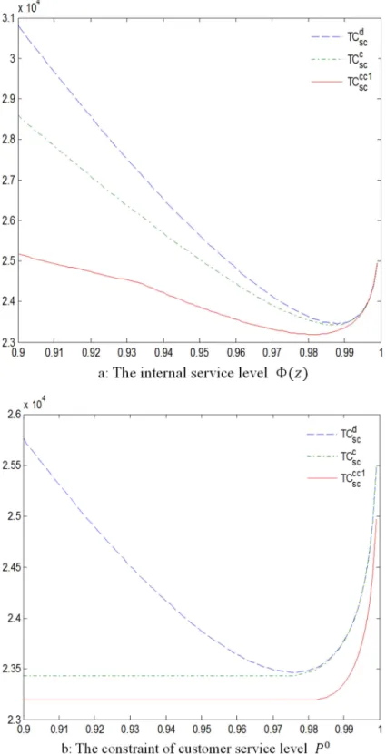
5.2. The Impact of Service Level
From the above analysis, we find both CCRP-1 and CCRP-2 can lower SC cost and CCRP-1 is more efficient, when ℎ =35, 25, 100 and 350. So we should choose CCRP-1 under these settings. To analyze the impacts of service level, we set Φ in the range of 90% and 99.9999%, and results are shown in figure 2 (a). Similar range is set for , with results given in figure 2 (b).
Figure 2 (a) analyzes the changes of SC cost of DRP, CRP
and CCRP-1, as Φ ranges from 90% to 99.99%. Result shows that SC costs of the three strategies first decrease with Φ and then increase. However, the inflection points of the three cost curves are different, and that of CCRP-1 is much lower than those of others. The lowest SC cost of CCRP-1 is 23193 at Φ 98.1%, which is much lower than those of other policies.
The impacts of on the SC costs of DRP, CRP and CCRP-1 are different from those of Φ( ), as shown in figure 2 (b). We find that a low has not effect on the SC costs of CRP and CCRP (see the flat lines). However, the curves have significantly gone up at a much higher level of . We also find the effect of on DRP is similar to that of
Φ( ), due to Φ( ) = . Finally, the inflection point of CCRP1 satisfies Φ( M ∗) = , and it is much higher than that of CRP.
From our analysis, we conclude that regardless of the service level, the CCRP-1 invariably dominates other policies.
5.3. The Comparative Analysis of Parameters Effects
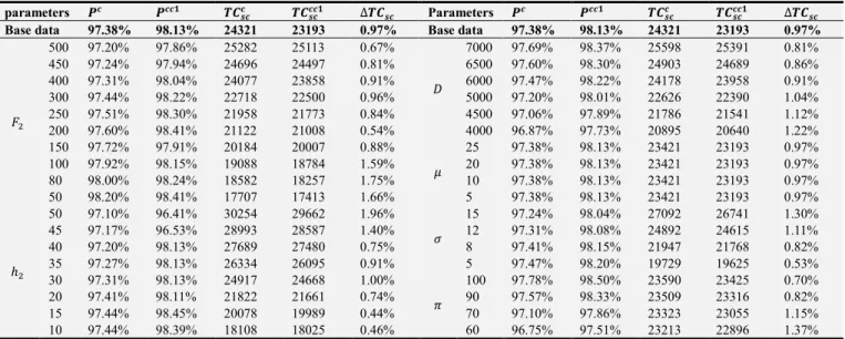
In this section, the impacts of parameters on service level and SC cost under different replenishment strategies are analyzed. We omit the analysis of DRP as CRP always outperforms DRP. Since the parameter effects on both CCRP-1 and CCRP-2 are similar, we only analyze CCRP-1. Therefore, we only compare the parameter effects on CRP and CCRP-1. For ease of explanation and without loss of generality, we analyze the effects of and ℎ , and let = 95%, ℎ = 35, and = 100. Results are summarized in Table 1, where s123M denotes the cost advantage of CCRP-1, i.e. tuvwwtuxtuvwwwP
vww ∗ 100%.
Table 1. The effects of parameters.
parameters yz yzzZ {|z}z {|}zzzZ ∆{|}z Parameters yz yzzZ {|z}z {|}zzzZ ∆{|}z Base data 97.38% 98.13% 24321 23193 0.97% Base data 97.38% 98.13% 24321 23193 0.97%
500 97.20% 97.86% 25282 25113 0.67%
G
7000 97.69% 98.37% 25598 25391 0.81%
450 97.24% 97.94% 24696 24497 0.81% 6500 97.60% 98.30% 24903 24689 0.86%
400 97.31% 98.04% 24077 23858 0.91% 6000 97.47% 98.22% 24178 23958 0.91%
300 97.44% 98.22% 22718 22500 0.96% 5000 97.20% 98.01% 22626 22390 1.04%
250 97.51% 98.30% 21958 21773 0.84% 4500 97.06% 97.89% 21786 21541 1.12%
200 97.60% 98.41% 21122 21008 0.54% 4000 96.87% 97.73% 20895 20640 1.22%
150 97.72% 97.91% 20184 20007 0.88% 25 97.38% 98.13% 23421 23193 0.97%
100 97.92% 98.15% 19088 18784 1.59% 20 97.38% 98.13% 23421 23193 0.97%
80 98.00% 98.24% 18582 18257 1.75% 10 97.38% 98.13% 23421 23193 0.97%
50 98.20% 98.41% 17707 17413 1.66% 5 97.38% 98.13% 23421 23193 0.97%
ℎ
50 97.10% 96.41% 30254 29662 1.96% 15 97.24% 98.04% 27092 26741 1.30%
45 97.17% 96.53% 28993 28587 1.40% 12 97.31% 98.08% 24892 24615 1.11%
40 97.20% 98.13% 27689 27480 0.75% 8 97.41% 98.15% 21947 21768 0.82%
35 97.27% 98.13% 26334 26095 0.91% 5 97.47% 98.20% 19729 19625 0.53%
30 97.31% 98.13% 24917 24668 1.00%
B
100 97.78% 98.50% 23590 23425 0.70%
20 97.41% 98.11% 21822 21661 0.74% 90 97.57% 98.33% 23509 23316 0.82%
15 97.44% 98.45% 20078 19989 0.44% 70 97.10% 97.86% 23323 23055 1.15%
10 97.44% 98.39% 18108 18025 0.46% 60 96.75% 97.51% 23213 22896 1.37%
Table 1 shows that when the parameters decrease, the expected SC cost of CRP and CCRP-1 will decrease. However, theses parameters have different effects on customer service level and SC. Note that customer service levels of CRP and CCRP1 increase with G and B, and decrease with . The cost advantage of CCRP-1 increases with , and decreases with B, meanwhile there is no clear relationship between cost and G. This is because varying G in CCRP-1 may cause the change of X, which leads to the variation in SC cost. The reason why cost advantage deteriorates with B is that the number of expected backorder in the coordinated replenishment cycle of CCRP-1 is larger than that in CRP. However, CCRP-1 still outperforms CRP, even when B is much larger. The effect of on the cost shows that CCRP-1 is more efficient in hedging high demand risk.
Results also show that component parameters ( and ℎ) have different effects on customer service level and cost advantage. M increases with the decreases of and ℎ , due to the trade off between service level and cost. However, the impacts of and ℎ on MM are much more complex. MM increases as and ℎ decrease, but only when they vary within a certain range. If the change of or ℎ is too large, the integer X will change accordingly. The effects of and ℎ on cost advantage of CCRP-1 is similar to that of MM ,
and the cost of CCRP-1 may even become larger than CRP as analyzed in Subsection 5.1.
6. Summary and Conclusions
In assembly systems, shortage of one or several components may discontinue the production process and results in huge loss. Joint coordination of material flows is critical for SC efficiency. Many organizations in different sectors have acknowledged the importance of synchronizing the material flow in supply chain, particularly for automotive and electronic sectors. This paper studies the coordination replenishment policies in an assembly system. We examine the replenishment coordination mechanism of a supply-hub, and propose three different policies to identify the most efficient replenishment policy. We conduct the feasibility study and assess the advantages of implementing coordinated replenishment policy. The key results are:
First, we prove that there exist optimal solutions in DRP and CRP. Although the expected SC cost of CCRP is not strictly convex in quantities and service level, it still has a global optimal solution.
especially by the replenishment cost (F) and component’s holding cost (h). Only when parameters satisfy a certain condition and CCRP-1 or CCRP-2 is correctly chosen, CCRP can reduce more cost than CRP. In addition, the larger the variation of lead time demand is, the more efficient of CCRP on reducing cost.
Third, when the required customer service level is low, it does not have impacts on the coordinated replenishment policy. Comparing with CRP, CCRP can significantly improve customer service level due to the decrease in the number of cross replenishment.
We have analyzed the feasibility and advantages of implementing coordinated replenishment policies. In the future, one can examine cost allocation (profit sharing) among SC partners, to ensure the cost charged to any SC member does not exceed that in DRP. In addition, one can extend the assembly line coordination mechanism analysis to multiple suppliers.
Acknowledgements
The author would like to thank the anonymous referees for their helpful comments and suggestions that greatly improved the presentation of this paper. This work was supported by Hubei Provincial Department of Education Humanities and social sciences research project (17G058), the Natural Sciences Foundation of China under Grants NSFC71471084, the key open-ended program of Wuhan Research Institute of Jianghan University (IWHS2016104), and Supported by the Funding under the Project of “Superiority Characteristic
Disciplines Group of Hubei Provincial Higher Universities-Urban Circle Economy and Industrial Integration Management”.
Appendix
Proof of Proposition 1. In DRP, both suppliers don’t share information, and the expected cost per unit time of supplier is increasing in inventory factor . So, to minimize cost, supplier choses the lowest service level that satisfies manufacturer’s demand, that is . Take the derivatives of equation /01234 with respect to , and we can get qN•0tuv'4
q6'N
5Q'
6'€ >0. So, /01234 is convex in , and the optimal value satisfies the first order condition.
Proof of Proposition 2. First, for any giving > 0, taking the first and second derivatives of the objective function
/0123M4 with respect to , we can get,
•/0123M4
• = −
G i + Rℎ;+ BS " ( − ) ( )#&$%' j
+ℎ2
• /0123M4
• =
2G i + Rℎ;+ BS " ( − ) ( )#&$%' j ‚ > 0
Obviously, Hessian matrix is greater than 0, so /0123M4 is joint convex in ( , ), and the optimal solutions satisfy the first order condition. Submit ( ∗, ∗) into /0123M4, we can rewrite the objective function,
/0123M( )4 = L J2Gℎ V + Rℎ;+ BS K ( − ) ( )# $%
&'
W + ℎ !
D
It is obvious that /0123M( )4 is convex in and the optimal solution satisfies the first order condition, which can be characterized as
L Gℎ Rℎ;+ BS " ( )#
$% &'
F2Gℎ i + Rℎ;+ BS " ( − ) ( )#&$%' j
− ℎ !
D
= 0
So, considering the customer service level constrain, the optimal value satisfies ∗= max ( , ).
Proof of the Proposition 3. Let superscript c and d denote CRP and DRP. Compare equations (3) and (6), and there is
" ( − ) ( )# > 0&$%' , so it is true than ∗M> ∗q. For any giving and M = q= , submit ∗ into the expected SC cost per unit time in CRP and DRP, and we can get /0123MM4 − /0123Mq4 = ∑ († − ‡ )D , where,
† = F2Gℎ 0 + (ℎ;+ B)4 " ( − ) ( )#&$%' > 0,
and
‡ = 2Gℎ + (ℎ;+ B)F5OQ''" ( − ) ( )# > 0&$%' .
Obviously, there is † − ‡ < 0, so it is true that † − ‡ < 0. It is easy to conclude that /0123MM4 < /0123Mq4.
‰•0tuvw4
‰6 −
5
6N d +fc +OP$cON, ‰ N•0tuvw4
‰6N 65€8d +fc9 >0, ‰•0tuvw4
‰c = − 5f
cN6+ON6, ‰ N•0tuvw4
‰cN =c5f€6> 0,
•/0123M4
• =
Rℎ + ℎ S −(cx )5c6 (ℎ + B) "&$%' ( )# −c65 0B "_`$%P$ab `N ( )# + ℎ "&P ( )#
_`P$ab `N 4, ‰N•0tuvw4
‰aN =(cx )5c6 (ℎ + B) ( ) +c65 (ℎ + B) R + S −c65 ℎ ( ).
For any giving , it is easy to know that /0123M4 is strictly convex in for any giving X > 0, and it is also strictly convex in X for any giving > 0. To prove /0123M4 is joint strictly in and X, we get the optimal value from the first
order condition, which can be expressed as, = J 5(e$
Š ‹) OP$cON
and X = FO5f
N6N. And then, submit the optimal values of
and X into the Hessian matrix about and X of /0123M4, which satisfies the equation Œ =cef ℎ > 0. Therefore,
/0123M4 is joint convex in and X, and get the optimal values satisfy the first order condition.
As we know, the inventory holding cost per unit per time is usually much less than the backorder cost per unit per time. So,
it is obviously that ‰N•0tu‰aNvw4> 0. In additional, there is > 0 and lim•→%‰•0tu‰avw4= (ℎ + ℎ ) > 0. Therefore, there is a unique optimal solution to minimize the expected SC cost per unit time.
Proof of Proposition 5. To prove /0123MM4 > /0123MMM 4, where the superscripts c and cc1 denote CRP and CCRP-1, we only need to prove + (ℎ + B) " ( − ) ( )# − .&$%
N > 0 .
Then we get when (ℎ + ℎ + B)‘"&P ( )# − ’ +
(ℎ + B)0"&N ( )# −"_`P$ab `N ( )# 4 > 0 is
satisfied, there is /0123MM4 > /0123MMM 4.
Proof of Proposition 6 is similar to the proof of Proposition 4, and Proof of Proposition 7 is similar to the proof of Proposition 5, which are omitted.
References
[1] Song J. S, Zipkin P. Supply chain operations: assemble-to-order systems. A. G. de Kok, S. C. Graves, eds. Handbooks in Operation Research and Management Science, 11. Supply Chain Management. Elsevier, Amsterdam, The Netherlands, 2003.
[2] Shah J, Goh M. Setting operating policies for supply-hubs. International Journal of Production Economics, 2006, 100 (2), 239–252.
[3] Guruprasad P, Chen Z. L. Joint cyclic production and delivery scheduling in a two-stage supply chain. International Journal of Production Economics, 2009, 119 (1), 55–74.
[4] Timmer J, Chessa M, Boucherie R. J. Cooperation and game-theoretic cost allocation in stochastic inventory models with continuous review. European Journal of Operational Research, 2013, 231 (3), 567–576.
[5] Khouja M, Goyal S. A review of the joint replenishment problem literature: 1989-2005. European Journal of Operational Research, 2008, 186 (1): 1-16.
[6] Qu W. W, Bookbinder J. H, Iyogun P. Integrated inventory-transportation system with modified periodic policy for multiple products. European Journal of Operational Research, 1999, 115:254-269.
[7] Minner S, Silver E. A. Multi-product batch replenishment strategies under stochastic demand and a joint capacity constraint. IIE Transactions, 2005, 37:469-479.
[8] De Boeck, L, Vandaele N. Analytical analysis of a generic assembly system. International Journal of Prduction Economics, 2011, 131, 107-114.
[9] De Boeck L, Vandaele N. Coordination and synchronization of material flows in supply chains: an analytical approach. International Journal of Production Economics, 2008, 116: 119-207.
[10] Sternatz J. The joint line balancing and material supply problem. International Journal of Production Economics, 2015, 159: 304-318.
[11] Antonio C. C, Pacifico M. P, Paolo S. Planning models for continuous supply of parts in assembly systems. Assembly Automation, 2015, 35 (1): 35-46.
[12] Simon E, Michel G. Scheduling in-house transport vehicles to feed parts to automotive assembly lines. European Journal of Operational Research, 2017, 260 (1): 255-267.
[13] Barnes E, Dai J, Deng S. On the Strategy of Supply-hubs for Cost Reduction and Responsiveness: White Paper on Electronics Supply Chain. Georgia Institute of Technology and National University of Singapore, 2000.
[14] Ma S. H, Gong F. M. Collaborative decision of distribution lot-sizing among suppliers based on supply-hub. Industrial Engineering and Management, 2009, 14 (2): 1-9.
[15] Li S. Y, Zhang D. Z, Jin F. P. Base inventory cooperation strategy of multi-parts with supply-hub. International Journal of Business and Management, 2013, 8 (20): 96-104.
[17] Zhong Jin-Hong, Jiang Rui-Xuan, and Zheng Gui. Multi-item distribution policies with supply hub and lateral transshipment. Mathematical Problems in Engineering, 2015, Article ID 702482, 12 pages, http://dx.doi.org/10.1155/2015/702482. [18] Zhang Ling-rong, Zhang Xing-long, Zhao Gan. Collaborative
replenishment decision based on supply-hub in the condition of uncertain demand. Systems Engineering, 2016, 34 (10): 98-107.
[19] Zhang Libin, Cheng Yaorong, Liang Jiajia. Mechanism of leader-follower distribution decision of the suppliers with the supply hub. Journal of Systems & Management, 2017, 26 (3): 577-582.
[20] Chen Jianhua, Li Li, Yang Huan. Simulation model of buffer inventory control in ATO supply chain based on supply-hub. Journal of Wuhan University of Technology (Transportation Science & Engineering), 2018, 42 (5): 738-743.
[21] Goyal, S. K. Note on: manufacturing cycle time determination for a multi-stage economic production quantity mode. Management Science, 1976, 23, 332–333.