Journal of Algebra Combinatorics Discrete Structures and Applications
On the spectral characterization of kite graphs
∗
Research Article
Sezer Sorgun, Hatice Topcu
Abstract: The Kite graph, denoted by Kitep,q is obtained by appending a complete graph Kp to a pendant vertex of a path Pq. In this paper, firstly we show that no two non-isomorphic kite graphs are cospectral w.r.t the adjacency matrix. Let Gbe a graph which is cospectral with Kitep,q and let w(G) be the clique number ofG. Then, it is shown thatw(G)≥p−2q+ 1. Also, we prove that Kitep,2 graphs are determined by their adjacency spectrum.
2010 MSC:05C50, 05C75
Keywords: Kite graph, Cospectral graphs, Clique number, Determined by adjacency spectrum
1.
Introduction
All of the graphs considered here are simple and undirected. LetG= (V, E)be a graph with vertex set V(G) = {v1, v2, . . . , vn} and edge set E(G). For a given graph F, if G does not contain F as an
induced subgraph, then Gis called F −f ree. A complete subgraph of G is aclique of G. The clique number of G is the number of the vertices in the largest clique ofG and it is denoted by w(G). Let
A(G) be the(0,1)-adjacency matrix of G and dk denotes the degree of the vertexvk. The polynomial
PA(G)(λ) = det(λI −A(G)) is the adjacency characteristic polynomial of G, where I is the identity matrix. Eigenvalues of the matrix A(G)are adjacency eigenvalues. Since A(G) is real and symmetric matrix, adjacency eigenvalues are all real numbers and could be ordered as λ1(A(G)) ≥ λ2(A(G)) ≥
. . . ≥ λn(A(G)). Adjacency spectrum of the graph G consists of the adjacency eigenvalues with their
multiplicities. The largest absolute value of the adjacency eigenvalues of a graph is known as itsadjacency spectral radius. Two graphs G andH are said to be cospectral if they have same spectrum (i.e., same characteristic polynomial). A graph G is determined by its adjacency spectrum, shortly DAS, if every graph cospectral with G w.r.t the adjacency matrix, is isomorphic to G. It is conjectured in [5] that almost all graphs are determined by their spectrum,DS for short. But it is difficult to show that a given
∗
This work was supported by the Nevsehir Haci Bektas Veli Univesity Coordinatorship of Scientific Research Projects (No. NEULUP15F17).
graph isDS. Up to now, some graphs are proved to beDS[1,2,4–11,13,15]. Recently, some papers have appeared in the literature that researchers focus on some special graphs (oftenly under some conditions) and prove that these special graphs areDS ornon-DS [1, 2,6–11, 13,15]. For a recent survey, one can see [5].
TheKite graph, denoted byKitep,q, is obtained by appending a complete graph withpverticesKp
to a pendant vertex of a path graph withqverticesPq. Ifq= 1, it is calledshort kite graph.
In this paper, firstly we obtain the characteristic polynomial of kite graphs and show that no two non-isomorphic kite graphs are cospectral w.r.t the adjacency matrix. Then for a given graphGwhich is cospectral withKitep,q, the clique number ofGisw(G)≥p−2q+ 1. Also we prove thatKitep,2graphs areDAS for allp.
2.
Preliminaries
First, we give some lemmas that will be used in the next sections of this paper.
Lemma 2.1. [8] Letx1 be a pendant vertex of a graphG andx2 be the vertex which is adjacent to x1.
Let G1 be the induced subgraph obtained from Gby deleting the vertex x1. Ifx1 andx2 are deleted, the
induced subgraph G2 is obtained. Then,
PA(G)(λ) =λPA(G1)(λ)−PA(G2)(λ)
Lemma 2.2. [4] For nxnmatrices AandB, followings are equivalent :
(i) A andB are cospectral
(ii) A andB have the same characteristic polynomial
(iii) tr(Ai) =tr(Bi)fori= 1,2, ..., n
Lemma 2.3. [4] For the adjacency matrix of a graph G, following parameters can be deduced from the spectrum;
(i) the number of vertices
(ii)the number of edges
(iii) the number of closed walks of any fixed length.
Theorem 2.4. [14] If a given connected graph G has the same order, same clique number and same spectral radius with Kitep,q then G is isomorphic to Kitep,q.
In the rest of the paper, we denote the number of subgraphs of a graphGwhich are isomorphic to complete graph K3byt(G).
Theorem 2.5. [14] For any integersp≥3andq≥1, if we denote the spectral radius ofA(Kitep,q)with
ρ(Kitep,q)then
p−1 + 1
p2 +
1
p3 < ρ(Kitep,q)< p−1 +
1 4p+
1
p2−2p
Theorem 2.6. [12] LetGbe a graph with n vertices, m edges and spectral radiusµ. IfGisKr+1−f ree,
then
µ≤
r
2m(r−1
r )
Lemma 2.7. [3](Interlacing Lemma) If G is a graph on n vertices with eigenvalues λ1(G)≥. . . ≥
λn(G) and H is an induced subgraph on m vertices with eigenvalues λ1(H) ≥ . . . ≥ λm(H), then for
i= 1, . . . , m
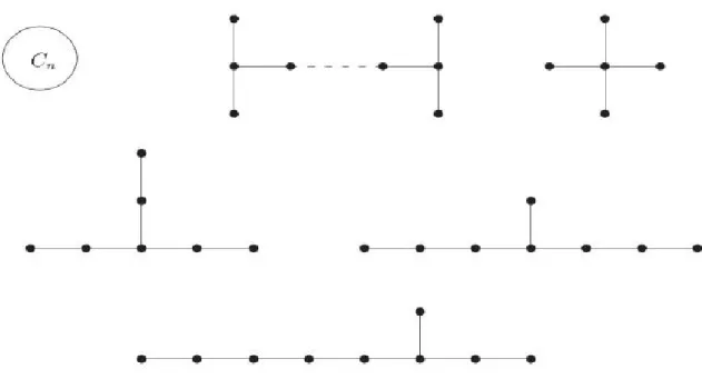
Lemma 2.8. [3] A connected graph with the largest adjacency eigenvalue less than 2 are precisely induced subgraphs of the Smith graphs shown in Figure 1.
Figure 1. Smith graphs
3.
Characteristic polynomial of kite graphs
We use the method similar to that given in [8] to obtain the general form of characteristic polynomials ofKitep,q graphs. Obviously, if we delete the vertex with one degree from short kite graph, the induced
subgraph will be the complete graphKp. Then, by deleting the vertex with one degree and its adjacent
vertex, we obtain the complete graphKp−1withp−1 vertices. From Lemma 2.1, we get
PA(Kitep,1)(λ) = λPA(Kp)(λ)−PA(Kp−1)(λ)
= λ(λ−p+ 1)(λ+ 1)p−1−[(λ−p+ 2)(λ+ 1)p−2] = (λ+ 1)p−2[(λ2−λp+λ)(λ+ 1)−λ+p−2] = (λ+ 1)p−2[λ3−(p−2)λ2−λp+p−2].
Similarly for Kitep,2, induced subgraphs will be Kitep,1andKp respectively. By Lemma 2.1, we get
PA(Kitep,2)(λ) = λPA(Kitep,1)(λ)−PA(Kp))(λ)
= λ(λPA(Kp)(λ)−PA(Kp−1)(λ))−PA(Kp))(λ) = (λ2−1)PA(Kp)(λ)−λPA(Kp−1)(λ).
By using these polynomials, we calculate the characteristic polynomial of Kitep,q wheren=p+q.
Again, by Lemma 2.1 we have
Coefficients of above equation areb1=−1, a1=λ. Simultaneously, we get
PA(Kitep,2)(λ) = (λ 2−1)P
A(Kp)(λ)−λPA(Kp−1)(λ).
and coefficients of above equation areb2=−a1=−λ,a2=λa1−1 =λ2−1. Then for Kitep,3, we have
PA(Kitep,3)(λ) = λPA(Kitep,2)(λ)−PA(Kitep,1))(λ)
= (λ(λ2−1)−λ)PA(Kp)(λ)−((λ
2−1)P
A(Kp−1)(λ))
and coefficients of above equation are b3 =−a2 =−(λ2−1), a3 = λa2−a1 = λ(λ2−1)−λ. In the following steps, forn≥3, an =λan−1−an−2. From this difference equation, we get
an= n
X
k=0
(λ+ √
λ2−4
2 )
k(λ−
√
λ2−4
2 )
n−k
Now, letλ= 2cosθandu=eiθ. Then, we have
an= n
X
k=0
u2k−n =u
−n(1−u2n+2)
1−u2
and by calculation the characteristic polynomial of any kite graph Kitep,q wheren=p+qis
PA(Kitep,q)(u+u
−1) = a
n−pPA(Kp)(u+u
−1)−a
n−p−1PA(Kp−1)(u+u −1)
= u
−n+p(1−u2n−2p+2)
1−u2 .((u+u
−1−p+ 1).(u+u−1+ 1)p−1)
−u
−n+p+1(1−u2n−2p+4)
1−u2 .((u+u
−1−p+ 2).(u+u−1+ 1)p−2)
= u
−n+p(1 +u−u−1)p−2
1−u2 [(2−p).(1 +u
−1
−u2n−2p+2−u2n−2p+3)
+(u−2−u2n−2p+4)]
= u
−q(1 +u−u−1)p−2
1−u2 [(2−p).(1 +u
−1−u2q+2−u2q+3)
+(u−2−u2q+4)].
Theorem 3.1. No two non-isomorphic kite graphs have the same adjacency spectrum.
Proof. Assume that there are two cospectral kite graphs with number of vertices respectively,p1+q1 and p2+q2. Since they are cospectral, they must have same number of vertices and same characteristic polynomials. Hence, n=p1+q1=p2+q2and we get
PA(Kitep1,q1)(u+u
−1) =P
A(Kitep2,q2)(u+u −1)
i.e.,
u−n+p1(1 +u−u−1)p1−2
1−u2 [(2−p1).(1 +u
−1−u2n−2p1+2−u2n−2p1+3)
+(u−2−u2n−2p1+4)]
= u
−n+p2(1 +u−u−1)p2−2
1−u2 [(2−p2).(1 +u
−1
−u2n−2p2+2−u2n−2p2+3)
i.e.,
up1.(1 +u−u−1)p1.[(2−p
1).(1 +u−1−u2n−2p1+2−u2n−2p1+3)
+(u−2−u2n−2p1+4)]
= up2.(1 +u−u−1)p2.[(2−p
2).(1 +u−1−u2n−2p2+2−u2n−2p2+3)
+(u−2−u2n−2p2+4)]
Letp1> p2. It follows thatn−p2> n−p1. Then, we have
up1−p2.(1 +u−u−1)p1−p2{[(2−p
1).(1 +u−1−u2n−2p1+2−u2n−2p1+3)
+(u−2−u2n−2p1+4)]−[(2−p
2).(1 +u−1−u2n−2p2+2−u2n−2p2+3)
+(u−2−u2n−2p2+4)]}= 0
By using the fact that u6= 0and1 +u+u−16= 0, we get
f(u) = [(2−p1).(1 +u−1−u2n−2p1+2−u2n−2p1+3) + (u−2−u2n−2p1+4)]
−[(2−p2).(1 +u−1−u2n−2p2+2−u2n−2p2+3) + (u−2−u2n−2p2+4)]
= 0
Sincef(u) = 0, the derivation of(2n−2p2+ 5)th off equals to zero again. Thus, we have
[(p1−2)(2n−2p2+ 4)!(u−2n+2p2−6)]−[(p2−2).(2n−2p2+ 4)!(u−2n+2p2−6)] = 0
i.e.,
[(p1−2)−(p2−2)].(u−2n+2p2−6) = 0
i.e.,
p1=p2
sinceu6= 0. This is a contradiction with our assumption that isp1> p2. Forp2> p1, we get the similar contradiction. Sop1 must be equal top2. Hence q1=q2and these graphs are isomorphic.
4.
Spectral characterization of Kite
p,
2
graphs
Lemma 4.1. LetGbe a graph which is cospectral with Kitep,q. Then we get
w(G)≥p−2q+ 1.
Proof. SinceGis cospectral withKitep,q, from Lemma 2.3,Ghas the same number of vertices, same
number of edges and same spectrum with Kitep,q. So, ifGhasnvertices andm edges, n=p+qand
m=
p
2
+q= p2−p2+2q. Also,ρ(G) =ρ(Kitep,q). From Theorem 2.6, we say that if µ >
q
2m(r−1
r )
thenGisn’tKr+1−f ree. It means that,GcontainsKr+1 as an induced subgraph. Now, we claim that forr < p−2q,
q
2m(r−r1)< ρ(G). By Theorem 2.5, we’ve already known that p−1 + p12 + 1
p3 < ρ(G). Hence, we need to show that
q
2m(r−r1)< p−1 + p12 + 1
(
r
2m(r−1
r ))
2
−(p−1 + 1
p2 +
1
p3)
2 = (p2
−p+ 2q)(r−1)−r(p−1 + 1
p2 +
1
p3) 2
= (p2−p+ 2q)(r−1)−
(r(p
2+p3)
p5 )(2(p−1) +
(p2+p3)
p5 )
= (pr−p2+p+ (2q−1)r−2q)−
(r(p
2+p3)
p5 )(2(p−1) +
(p2+p3)
p5 )
By the help ofMathematica, forr < p−2qwe can see
(pr−p2+p+ (2q−1)r−2q)−(r(p
2+p3)
p5 )(2(p−1) +
(p2+p3)
p5 )<0
i.e.,
(
r
2m(r−1
r ))
2−(p−1 + 1
p2+
1
p3) 2<0
i.e.,
(
r
2m(r−1
r ))
2<(p−1 + 1
p2 +
1
p3) 2
Sinceq2m(r−r1)>0 andp−1 +p12 + 1
p3 >0, we get
r
2m(r−1
r )< p−1 +
1
p2 +
1
p3 < ρ(G).
Thus, we proved our claim and so GcontainsKr+1 as an induced subgraph such that r < p−2q. Consequently,w(G)≥p−2q+ 1.
Theorem 4.2. Kitep,2 graphs are determined by their adjacency spectrum for allp.
Proof. Ifp= 1orp= 2,Kitep,2graphs are actually the path graphsP3or P4. Also ifp= 3, then we obtain the lollipop graph H5,3. As is known, these graphs are already DAS [8]. Hence we will continue
our proof forp≥4. Adjacency characteristic polynomial ofKitep,2 is as below,
PA(Kitep,2)(λ) = (λ+ 1)
p−2[λ4+ (2−p)λ3−(p+ 1)λ2+ (2p−4)λ+p−1]
By calculation, for the adjacency eigenvalues ofKitep,2, we obtain the following facts;
p−1 < λ1(A(Kitep,2)) < p, 0 < λ2(A(Kitep,2)) < 2, λ3(A(Kitep,2)) < 0, λ4(A(Kitep,2)) = . . . =
λp+1(A(Kitep,2)) =−1andλp−1(A(Kitep,2))<−1.
For a given graphGwith nvertices and medges, assume that Gis cospectral withKitep,2. Then by Lemma 2.3, n=p+ 2,m=
p
2
+ 2 = p2−2p+4 andt(G) =t(Kitep,2) =
p
3
Lemma 4.1,w(G)≥p−2q+ 1. Whenq= 2,w(G)≥p−3 =n−5. It’s well-known that complete graph
Kn isDS. Sow(G)6=n. Ifw(G) =n−1 =p+ 1, thenGcontains at least one clique with sizep−1. It
means that the edge number of Gis greater than or equal to
p+ 1 2
. But it is a contradiction since
p+ 1 2
>
p
2
+ 2 =m. Hence, w(G)6=n−1. Because of these facts, we getp−3 ≤w(G)≤p.
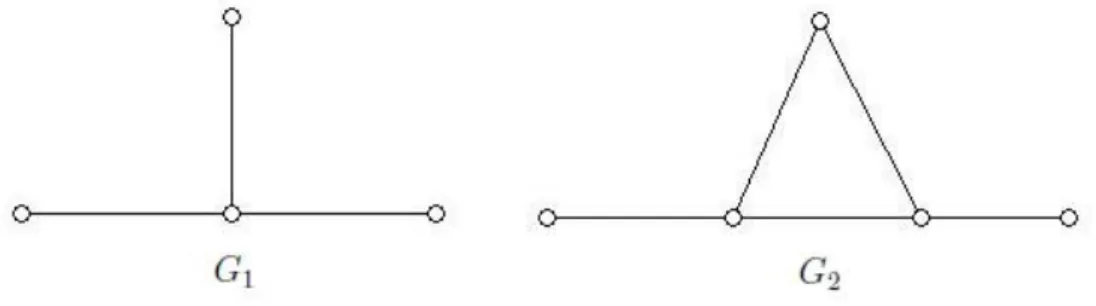
From interlacing lemma, Gcan not contain the graphs in the following figure as an induced subgraph because λ3(G1) =λ3(G2) = 0.
Figure 2. Graphs G1 and G2
If G is disconnected, from Lemma 2.8, components of G except one of them must be induced subgraphs of Smith graphs. Clearly, this is impossible becauseG1is forbidden and any path graph (since they have symmetric eigenvalues) can not be a component of G. Hence Gmust be a connected graph. If w(G) =p, then by Theorem 2.4.,G∼=Kitep,2. So we continue for w(G) < p. Since w(G)≥p−3,
G contains at least one clique with size at leastp−3. This clique is denoted byKw(G). There may be at most five vertices out of the cliqueKw(G). Let us label these five vertices respectively with1,2,3,4,5 and call the set of these five vertices withA. So, we get |A| ≤5. Moreover, ∀i, j∈Awe geti∼j since
G1,G2are not induced subgraphs ofGand there is no isolated vertex inG. Then, we can say thatp≥6 sincew(G)≥p−3.
Fori∈A,xidenotes the number of adjacent vertices ofiinKw(G). By the fact thatp−1≥w(G)≥
p−3, for alli∈Awe say
xi≤w(G)− |A|+ 1 (1)
Also, xi∧j denotes the number of common adjacent vertices inKw(G) ofi and j such thati, j ∈Aand
i < j. Similarly, ifi∼j then
xi∧j≤w(G)− |A| (2)
Let ddenotes the number of edges between the vertices of A and Kw(G), alsoαdenotes the number of cliques with size 3 which are not contained byA orKw(G). Then, we get
m=
p
2
+ 2 =
w(G) 2
+
|A| 2
+d. (3)
Similarly, we get
t(G) =
p
3
=
w(G) 3
+
|A| 3
+α. (4)
On the other hand forαandd, we have
d=
|A|
X
i=1
and
α=
|A|
X i=1 xi 2 +X
i∼j
xi∧j. (6)
Ifw(G) =p−3then|A|= 5and sop≥8. Thus we have
d= 3p−14 (7)
and α= p 3 −
p−3 3
−10 =3p
2
2 − 15p
2 . (8)
From (1),(2),(5),(6) and (7) we have
α= 5 X i=1 xi 2 +X
i∼j
xi∧j ≤ 3
p−7 2 + 7 2 + 2 5 X i=1 xi = 3
p−7 2 + 7 2
+ 6p−28
= 3p
2−33p
2 + 77.
But obviously forp= 8this result gives contradiction. Also forp >8,
3p2−33p
2 + 77<
3p2−15p
2 =α.
So this is again a contradiction.
Ifw(G) =p−2 then|A|= 4and sop≥7. Thus we have
d= 2p−7
and α= p 3 −
p−2 3
−4 =p2−4p.
On the other hand we have
α= 4 X i=1 xi 2 +X
i∼j
xi∧j ≤ 2
p−5 2 + 3 2 + 2 4 X i=1 xi
= p2−7p+ 19.
Clearly forp≥7,
p2−7p+ 19< p2−4p=α.
So this is a contradiction.
Similarly, ifw(G) =p−1then|A|= 3and sop≥6. Hence we have
d=p−2
and
α=p
2−3p
Also we have
α=
3 X
i=1
xi
2
+X
i∼j
xi∧j ≤
p−3 2
+p−2
= p
2−5p
2 + 4.
Clearly forp≥6,
p2−5p
2 + 4<
p2−3p
2 =α.
Again we obtain a contradiction.
By all of these facts, we can conclude that our assumption is actually false, thenw(G)6< p. Hence
w(G) =pand so that by Theorem 2.4.,G∼=Kitep,2.
In the final of the paper, we give a conjecture below.
Conjecture 4.3. Forq >2, Kitep,q graphs are DAS.
Acknowledgment: The authors are grateful to the referees for many suggestions which led to an improved version of this paper.
References
[1] R. Boulet, B. Jouve, The lollipop graph is determined by its spectrum, Electron. J. Combin. 15(1) (2008) Research Paper 74, 43 pp.
[2] M. Camara, W. H. Haemers, Spectral characterizations of almost complete graphs, Discrete Appl. Math. 176 (2014) 19–23.
[3] M. D. Cvetkovic, P. Rowlinson, S. Simic, An Introduction to the Theory of Graph Spectra, Cambridge University Press, 2010.
[4] E.R. van Dam, W. H. Haemers, Which graphs are determined by their spectrum?, Linear Algebra Appl. 373 (2003) 241–272.
[5] E.R. van Dam, W. H. Haemers, Developments on spectral characterizations of graphs, Discrete Math. 309(3) (2009) 576–586.
[6] M. Doob, W. H. Haemers, The complement of the path is determined by its spectrum, Linear Algebra Appl. 356(1-3) (2002) 57–65.
[7] N. Ghareghani, G. R. Omidi, B. Tayfeh-Rezaie, Spectral characterization of graphs with index at mostp2 +√5, Linear Algebra Appl. 420(2-3) (2007) 483–486.
[8] W. H. Haemers, X. Liu, Y. Zhang, Spectral characterizations of lollipop graphs, Linear Algebra Appl. 428(11-12) (2008) 2415–2423.
[9] F. Liu, Q. Huang, J. Wang, Q. Liu, The spectral characterization of∞-graphs, Linear Algebra Appl. 437(7) (2012) 1482–1502.
[10] M. Liu, H. Shan, K. Ch. Das, Some graphs determined by their (signless) Laplacian spectra, Linear Algebra Appl. 449 (2014) 154–165.
[11] X. Liu, Y. Zhang, X. Gui, The multi-fan graphs are determined by their Laplacian spectra, Discrete Math. 308(18) (2008) 4267–4271.
[12] V. Nikiforov, Some inequalities for the largest eigenvalue of a graph, Combin. Probab. Comput. 11(2) (2002) 179–189.
[14] D. Stevanovic, P. Hansen, The minimum spectral radius of graphs with a given clique number, Electron. J. Linear Algebra. 17 (2008) 110–117.