Real-Time Dynamic Voltage Scaling for Low-Power
Embedded Operating Systems
Padmanabhan Pillai and Kang G. Shin
Real-Time Computing Laboratory
Department of Electrical Engineering and Computer Science The University of Michigan
Ann Arbor, MI 48109-2122, U.S.A.
fpillai,[email protected]
ABSTRACT
In recent years, there has been a rapid and wide spread of non-traditional computing platforms, especially mobile and portable com-puting devices. As applications become increasingly sophisticated and processing power increases, the most serious limitation on these devices is the available battery life. Dynamic Voltage Scaling (DVS) has been a key technique in exploiting the hardware characteristics of processors to reduce energy dissipation by lowering the supply voltage and operating frequency. The DVS algorithms are shown to be able to make dramatic energy savings while providing the nec-essary peak computation power in general-purpose systems. How-ever, for a large class of applications in embedded real-time sys-tems like cellular phones and camcorders, the variable operating frequency interferes with their deadline guarantee mechanisms, and DVS in this context, despite its growing importance, is largely overlooked/under-developed. To provide real-time guarantees, DVS must consider deadlines and periodicity of real-time tasks, requir-ing integration with the real-time scheduler. In this paper, we present a class of novel algorithms called real-time DVS (RT-DVS) that modify the OS’s real-time scheduler and task management service to provide significant energy savings while maintaining real-time deadline guarantees. We show through simulations and a working prototype implementation that these RT-DVS algorithms closely approach the theoretical lower bound on energy consumption, and can easily reduce energy consumption 20% to 40% in an embedded real-time system.
1.
INTRODUCTION
Computation and communication have been steadily moving to-ward mobile and portable platforms/devices. This is very evident in the growth of laptop computers and PDAs, but is also occur-ring in the embedded world. With continued miniaturization and increasing computation power, we see ever growing use of
The work reported in this paper is supported in part by the U.S. Airforce Office of Scientific Research under Grant AFOSR F49620-01-1-0120.
ful microprocessors running sophisticated, intelligent control soft-ware in a vast array of devices including digital camcorders, cellu-lar phones, and portable medical devices.
Unfortunately, there is an inherent conflict in the design goals be-hind these devices: as mobile systems, they should be designed to maximize battery life, but as intelligent devices, they need powerful processors, which consume more energy than those in simpler de-vices, thus reducing battery life. In spite of continuous advances in semiconductor and battery technologies that allow microprocessors to provide much greater computation per unit of energy and longer total battery life, the fundamental tradeoff between performance and battery life remains critically important.
Recently, significant research and development efforts have been made on Dynamic Voltage Scaling (DVS) [2, 4, 7, 8, 12, 19, 21, 22, 23, 24, 25, 26, 28, 30]. DVS tries to address the tradeoff between performance and battery life by taking into account two important characteristics of most current computer systems: (1) the peak computing rate needed is much higher than the average throughput that must be sustained; and (2) the processors are based on CMOS logic. The first characteristic effectively means that high performance is needed only for a small fraction of the time, while for the rest of the time, a low-performance, low-power processor would suffice. We can achieve the low performance by simply lowering the operating frequency of the processor when the full speed is not needed. DVS goes beyond this and scales the oper-ating voltage of the processor along with the frequency. This is possible because static CMOS logic, used in the vast majority of microprocessors today, has a voltage-dependent maximum operat-ing frequency, so when used at a reduced frequency, the processor can operate at a lower supply voltage. Since the energy dissipated per cycle with CMOS circuitry scales quadratically to the supply voltage (E /V
2
) [2], DVS can potentially provide a very large net energy savings through frequency and voltage scaling. In time-constrained applications, often found in embedded systems like cellular phones and digital video cameras, DVS presents a se-rious problem. In these real-time embedded systems, one cannot directly apply most DVS algorithms known to date, since chang-ing the operatchang-ing frequency of the processor will affect the exe-cution time of the tasks and may violate some of the timeliness guarantees. In this paper, we present several novel algorithms that incorporate DVS into the OS scheduler and task management ser-vices of a real-time embedded system, providing the energy sav-ings of DVS while preserving deadline guarantees. This is in sharp
contrast with the average throughput-based mechanisms typical of many current DVS algorithms. In addition to detailed simulations that show the energy-conserving benefits of our algorithms, we also present an actual implementation of our mechanisms, demonstrat-ing them with measurements on a workdemonstrat-ing system. To the best of our knowledge, this is one of the first working implementations of DVS, and the first implementation of Real-Time DVS (RT-DVS). In the next section, we present details of DVS, real-time schedul-ing, and our new RT-DVS algorithms. Section 3 presents the sim-ulation results and provides insight into the system parameters that most influence the energy-savings potential of RT-DVS. Section 4 describes our implementation of RT-DVS mechanisms in a work-ing system and some measurements obtained. Section 5 presents related work and puts our work in a larger perspective before we close with our conclusions and future directions in Section 6.
2.
RT-DVS
To provide energy-saving DVS capability in a system requiring real-time deadline guarantees, we have developed a class of RT-DVS algorithms. In this section, we first consider RT-DVS in general, and then discuss the restrictions imposed in embedded real-time systems. We then present RT-DVS algorithms that we have devel-oped for this time-constrained environment.
2.1
Why DVS?
Power requirements are one of the most critical constraints in mo-bile computing applications, limiting devices through restricted power dissipation, shortened battery life, or increased size and weight. The design of portable or mobile computing devices involves a tradeoff between these characteristics. For example, given a fixed size or weight for a handheld computation device/platform, one could design a system using a low-speed, low-power processor that provides long battery life, but poor performance, or a system with a (literally) more powerful processor that can handle all computa-tional loads, but requires frequent battery recharging. This simply reflects the cost of increasing performance — for a given technol-ogy, the faster the processor, the higher the energy costs (both over-all and per unit of computation).
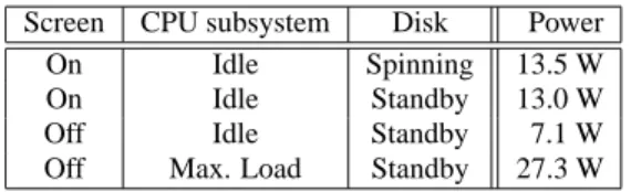
The discussion in this paper will generally focus on the energy con-sumption of the processor in a portable computation device for two main reasons. First, the practical size and weight of the device are generally fixed, so for a given battery technology, the avail-able energy is also fixed. This means that only power consumption affects the battery life of the device. Secondly, we focus partic-ularly on the processor because in most applications, the proces-sor is the most energy-consuming component of the system. This is definitely true on small handheld devices like PDAs [3], which have very few components, but also on large laptop computers [20] that have many components including large displays with back-lighting. Table 1 shows measured power consumption of a typical laptop computer. When it is idle, the display backlighting accounts for a large fraction of dissipated power, but at maximum compu-tational load, the processor subsystem dominates, accounting for nearly 60% of the energy consumed. As a result, the design prob-lem generally boils down to a tradeoff between the computational power of the processor and the system’s battery life.
One can avoid this problem by taking advantage of a feature very common in most computing applications: the average computa-tional throughput is often much lower than the peak computacomputa-tional capacity needed for adequate performance. Ideally, the processor
Screen CPU subsystem Disk Power On Idle Spinning 13.5 W
On Idle Standby 13.0 W
Off Idle Standby 7.1 W
Off Max. Load Standby 27.3 W
Table 1: Power consumption measured on Hewlett-Packard N3350 laptop computer
would be “sized” to meet the average computational demands, and would have low energy costs per unit of computation, thus provid-ing good battery life. Durprovid-ing the (relatively rare) times when peak computational load is imposed, the higher computational through-put of a more sophisticated processor would somehow be “config-ured” to meet the high performance requirement, but at a higher energy cost per unit of computation. Since the high-cost cycles are applied for only some, rather than all, of the computation, the energy consumption will be lower than if the more powerful pro-cessor were used all of the time, but the performance requirements are still met.
One promising mechanism that provides the best of both low-power and high-performance processors in the same system is DVS [30]. DVS relies on special hardware, in particular, a programmable DC-DC switching voltage regulator, a programmable clock generator, and a high-performance processor with wide operating ranges, to provide this best-of-both-worlds capability. In order to meet peak computational loads, the processor is operated at its normal volt-age and frequency (which is also its maximum frequency). When the load is lower, the operating frequency is reduced to meet the computational requirements. In CMOS technology, used in virtu-ally all microprocessors today, the maximum operating frequency increases (within certain limits) with increased operating voltage, so when the processor is run slower, a reduced operating voltage suffices [2]. A second important characteristic is that the energy consumed by the processor per clock cycle scales quadratically with the operating voltage (E /V
2
) [2], so even a small change in voltage can have a significant impact on energy consumption. By dynamically scaling both voltage and frequency of the proces-sor based on computation load, DVS can provide the performance to meet peak computational demands, while on average, providing the reduced power consumption (including energy per unit compu-tation) benefits typically available on low-performance processors.
2.2
Real-time issues
For time-critical applications, however, the scaling of processor fre-quency could be detrimental. Particularly in real-time embedded systems like portable medical devices and cellular phones, where tasks must be completed by some specified deadlines, most rithms for DVS known to date cannot be applied. These DVS algo-rithms do not consider real-time constraints and are based on solely average computational throughput [7, 23, 30]. Typically, they use a simple feedback mechanism, such as detecting the amount of idle time on the processor over a period of time, and then adjust the fre-quency and voltage to just handle the computational load. This is very simple and follows the load characteristics closely, but cannot provide any timeliness guarantees and tasks may miss their execu-tion deadlines. As an example, in an embedded camcorder con-troller, suppose there is a program that must react to a change in a sensor reading within a 5 ms deadline, and that it requires up to 3 ms of computation time with the processor running at the maxi-mum operating frequency. With a DVS algorithm that reacts only
EDF test ():
if (C1=P1++Cn=Pn) return true;
else return false; RM test ():
if (8T i
2fT 1
;:::;T n
jP 1
P n
g
dPi=P1eC1++dPi=PieCiPi)
return true; else return false; select frequency:
use lowest frequencyf i
2ff 1
;:::;f m
jf 1
<<f m
g
such that RM test(fi=fm) or EDF test(fi=fm) is true.
Figure 1: Static voltage scaling algorithm for EDF and RM schedulers
to average throughput, if the total load on the system is low, the processor would be set to operate at a low frequency, say half of the maximum, and the task, now requiring 6 ms of processor time, cannot meet its 5 ms deadline. In general, none of the average throughput-based DVS algorithms found in literature can provide real-time deadline guarantees.
In order to realize the reduced energy-consumption benefits of DVS in a real-time embedded system, we need new DVS algorithms that are tightly-coupled with the actual real-time scheduler of the oper-ating system. In the classic model of a real-time system, there is a set of tasks that need to be executed periodically. Each task,T
i, has
an associated period,P
i, and a worst-case computation time, C
i.
1.
The task is released (put in a runnable state) periodically once ev-eryPitime units (actual units can be seconds or processor cycles
or any other meaningful quanta), and it can begin execution. The task needs to complete its execution by its deadline, typically de-fined as the end of the period [18], i.e., by the next release of the task. As long as each taskT
iuses no more than C
icycles in each
invocation, a real-time scheduler can guarantee that the tasks will always receive enough processor cycles to complete each invoca-tion in time. Of course, to provide such guarantees, there are some conditions placed on allowed task sets, often expressed in the form of schedulability tests. A real-time scheduler guarantees that tasks will meet their deadlines given that:
C1. the task set is schedulable (passes schedulability test), and C2. no task exceeds its specified worst-case computation bound.
DVS, when applied in a real-time system, must ensure that both of these conditions hold.
In this paper, we develop algorithms to integrate DVS mechanisms into the two most-studied real-time schedulers, Rate Monotonic (RM) and Earliest-Deadline-First (EDF) schedulers [13, 14, 17, 18, 27]. RM is a static priority scheduler, and assigns task prior-ity according to period — it always selects first the task with the shortest period that is ready to run (released for execution). EDF is a dynamic priority scheduler that sorts tasks by deadlines and al-ways gives the highest priority to the released task with the most
1
Although not explicit in the model, aperiodic and sporadic tasks can be handled by a periodic or deferred server [16] For non-real-time tasks, too, we can provision processor non-real-time using a similar periodic server approach.
0 5 10 15
0 5 10 15
0 5 10 15
0.50 0.75 1.00
0.50 0.75 1.00
0.50 0.75 1.00
deadline T3 misses
T1 T2 T3 T1 T2
T2
T2 T3
T1 T1 T3
T1 T2 T1 T2
ms
ms ms
frequency
frequency
frequency
Static EDF uses 0.75
Static RM uses 1.0
Static RM fails at 0.75
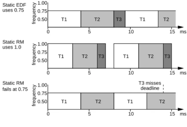
Figure 2: Static voltage scaling example
Task Computing Time Period
1 3 ms 8 ms
2 3 ms 10 ms
3 1 ms 14 ms
Table 2: Example task set, where computing times are specified at the maximum processor frequency
imminent deadline. In the classical treatments of these schedulers [18], both assume that the task deadline equals the period (i.e., the task must complete before its next invocation), that scheduling and preemption overheads are negligible,2 and that the tasks are
inde-pendent (no task will block waiting for another task). In our design of DVS to real-time systems, we maintain the same assumptions, since our primary goal is to reduce energy consumption, rather than to derive general scheduling mechanisms.
In the rest of this section, we present our algorithms that perform DVS in time-constrained systems without compromising deadline guarantees of real-time schedulers.
2.3
Static voltage scaling
We first propose a very simple mechanism for providing voltage scaling while maintaining real-time schedulability. In this mecha-nism we select the lowest possible operating frequency that will al-low the RM or EDF scheduler to meet all the deadlines for a given task set. This frequency is set statically, and will not be changed unless the task set is changed.
To select the appropriate frequency, we first observe that scaling the operating frequency by a factor (0 < 1) effectively
results in the worst-case computation time needed by a task to be scaled by a factor1=, while the desired period (and deadline)
re-mains unaffected. We can take the well-known schedulability tests for EDF and RM schedulers from the real-time systems literature, and by using the scaled values for worst-case computation needs of the tasks, can test for schedulability at a particular frequency. The necessary and sufficient schedulability test for a task set under ideal EDF scheduling requires that the sum of the worst-case
uti-lizations (computation time divided by period) be less than one, i.e.,
C1=P1++Cn=Pn 1[18]. Using the scaled computation
time values, we obtain the EDF schedulability test with frequency
2
We note that one could account for preemption overheads by computing the worst-case preemption sequences for each task and adding this overhead to its worst-case computation time.
0 5 10 15 0.50
0.75 1.00
ms
frequency T1 T2 T3 T1 T2 T3
0.546 0.621 0.421 0.296
0.421 0.496 0.296 0.296
i
ΣU =0.746
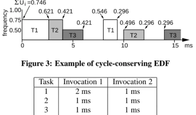
Figure 3: Example of cycle-conserving EDF
Task Invocation 1 Invocation 2
1 2 ms 1 ms
2 1 ms 1 ms
3 1 ms 1 ms
Table 3: Actual computation requirements of the example task set (assuming execution at max. frequency)
scaling factor:
C1=P1++Cn=Pn
Similarly, we start with the sufficient (but not necessary) condition for schedulability under RM scheduling [13] and obtain the test for a scaled frequency (see Figure 1). The operating frequency se-lected is the lowest one for which the modified schedulability test succeeds. The voltage, of course, is changed to match the oper-ating frequency. Assume that the operoper-ating frequencies and the corresponding voltage settings available on the particular hardware platform are specified in a table provided to the software. Figure 1 summarizes the static voltage scaling for EDF and RM schedul-ing, where there aremoperating frequenciesf1;:::;fmsuch that f1 <f2<<fm.
Figure 2 illustrates these mechanisms, showing sample worst-case execution traces under statically-scaled EDF and RM scheduling. The example uses the task set in Table 2, which indicates each task’s period and worst-case computation time, and assumes that three normalized, discrete frequencies are available (0.5, 0.75, and 1.0). The figure also illustrates the difference between EDF and RM (i.e., deadline vs. rate for priority), and shows that statically-scaled RM cannot reduce frequency (and therefore reduce voltage and conserve energy) as aggressively as the EDF version.
As long as for some available frequency, the task set passes the schedulability test, and as long as the tasks use no more than their scaled computation time, this simple mechanism will ensure that frequency and voltage scaling will not compromise timely execu-tion of tasks by their deadlines. The frequency and voltage set-ting selected are static with respect to a particular task set, and are changed only when the task set itself changes. As a result, this mechanism need not be tightly-coupled with the task management functions of the real-time operating system, simplifying implemen-tation. On the other hand, this algorithm may not realize the full potential of energy savings through frequency and voltage scaling. In particular, the static voltage scaling algorithm does not deal with situations where a task uses less than its worst-case requirement of processor cycles, which is usually the case. To deal with this com-mon situation, we need more sophisticated, RT-DVS mechanisms.
2.4
Cycle-conserving RT-DVS
Although real-time tasks are specified with worst-case computation requirements, they generally use much less than the worst case on most invocations. To take best advantage of this, a DVS mechanism could reduce the operating frequency and voltage when tasks use less than their worst-case time allotment, and increase frequency
select frequency():
use lowest freq.fi2ff1;:::;fmjf1<<fmg
such thatU 1
++U n
f i
=f m
upon task release(Ti):
setU ito
C i
=P i;
select frequency(); upon task completion(T i):
setUitocci=Pi;
/*cciis the actual cycles used this invocation */
select frequency();
Figure 4: Cycle-conserving DVS for EDF schedulers
to meet the worst-case needs. When a task is released for its next invocation, we cannot know how much computation it will actu-ally require, so we must make the conservative assumption that it will need its specified worst-case processor time. When the task completes, we can compare the actual processor cycles used to the worst-case specification. Any unused cycles that were allot-ted to the task would normally (or eventually) be wasallot-ted, idling the processor. Instead of idling for extra processor cycles, we can devise DVS algorithms that avoid wasting cycles (hence “cycle-conserving”) by reducing the operating frequency. This is some-what similar to slack time stealing [15], except surplus time is used to run other remaining tasks at a lower CPU frequency rather than accomplish more work. These algorithms are tightly-coupled with the operating system’s task management services, since they may need to reduce frequency on each task completion, and increase frequency on each task release. The main challenge in designing such algorithms is to ensure that deadline guarantees are not vio-lated when the operating frequencies are reduced.
For EDF scheduling, as mentioned earlier, we have a very simple schedulability test: as long as the sum of the worst-case task uti-lizations is less than, the task set is schedulable when operating
at the maximum frequency scaled by factor. If a task completes
earlier than its worst-case computation time, we can reclaim the excess time by recomputing utilization using the actual computing time consumed by the task. This reduced value is used until the task is released again for its next invocation. We illustrate this in Figure 3, using the same task set and available frequencies as be-fore, but using actual execution times from Table 3. Here, each invocation of the tasks may use less than the specified worst-case times, but the actual value cannot be known to the system until after the task completes execution. Therefore, at each scheduling point (task release or completion) the utilization is recomputed using the actual time for completed tasks and the specified worst case for the others, and the frequency is set appropriately. The numerical val-ues in the figure show the total task utilizations computed using the information available at each point.
The algorithm itself (Figure 4) is simple and works as follows. Sup-pose a taskTicompletes its current invocation after usingccicycles
which are usually much smaller than its worst-case computation timeC
i. Since task T
iuses no more than cc
icycles in its current
invocation, we treat the task as if its worst-case computation bound werecc
i. With the reduced utilization specified for this task, we can
now potentially find a smaller scaling factor(i.e., lower operating
0.50 0.75 1.00
0 5 10 15
frequency
ms
0.50 0.75 1.00
0 5 10 15
frequency
ms
0.50 0.75 1.00
0 5 10 15
frequency
ms (a)
(b)
(c)
D1
D1 D2
D3
D3 D2
D1 D2 D3
time=0
time=2 time=0
T1
T2 T3
T1 T2 T3
T3 T2 T1
T3 T2 T1
T1 T2 T3 T1 T2 T3
0.50 0.75 1.00
0 5 10 15
frequency
ms
0.50 0.75 1.00
0 5 10 15
frequency
ms 0.50
0.75 1.00
0 5 10 15
(d)
(e)
(f)
D2 D3 D1
D2 D3
time=16 time=8
frequency
ms time=3.33
T1 T3
T1
T1
T1 T2
T3
T1 T2
T3
T2 T3 T2
T2
T3
T2 T3 T1
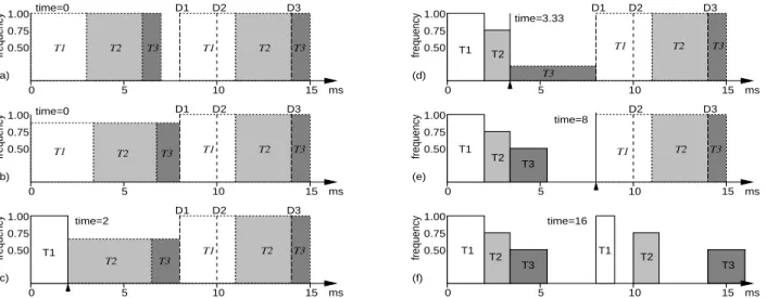
Figure 5: Example of cycle-conserving RM: (a) Initially use statically-scaled, worst-case RM schedule as target; (b) Determine minimum frequency so as to complete the same work by D1; rounding up to the closest discrete setting requires frequency 1.0; (c) After T1 completes (early), recompute the required frequency as 0.75; (d) Once T2 completes, a very low frequency (0.5) suffices to complete the remaining work by D1; (e) T1 is re-released, and now, try to match the work that should be done by D2; (f) Execution trace through time 16 ms.
assumefjis frequency set by static scaling algorithm
select frequency():
setsm= max cycles until next deadline();
use lowest freq.f i
2ff 1
;:::;f m
jf 1
<<f m
g
such that(d 1
++d n
)=s m
f i
=f m
upon task release(T i):
setcleft i
=C i;
setsm= max cycles until next deadline();
sets j=
s m
f j
=f m;
allocate cycles (s j);
select frequency(); upon task completion(T i):
setcleft i= 0;
setdi= 0;
select frequency(); during task execution(Ti):
decrementcleft i
andd i;
allocate cycles(k):
fori= 1 ton, Ti2fT1;:::;TnjP1Png
/* tasks sorted by period */ if (cleft
i <k)
setdi=cleft i;
setk=k-cleft i
; else
setdi=k;
setk= 0;
Figure 6: Cycle-conserving DVS for RM schedulers
given that the task set prior to this change was schedulable, the EDF schedulability test will continue to hold, andT
i(which has
com-pleted execution) will not violate its lowered maximum computing bound for the remainder of time until its deadline. Therefore, the task set continues to meet both conditions C1 and C2 imposed by the real-time scheduler to guarantee timely execution, and as a re-sult, deadline guarantees provided by EDF scheduling will continue to hold at least untilT
iis released for its next invocation. At this
point, we must restore its computation bound toCito ensure that
it will not violate the temporarily-lowered bound and compromise the deadline guarantees. At this time, it may be necessary to in-crease the operating frequency. At first glance, this algorithm does not appear to significantly reduce frequencies, voltages, and energy expenditure. However, since multiple tasks may be simultaneously in the reduced-utilization state, the total savings can be significant. We could use the same schedulability-test-based approach to de-signing a cycle-conserving DVS algorithm for RM scheduling, but as the RM schedulability test is significantly more complex (O(n
2 ),
wherenis the number of tasks to be scheduled), we will take a
dif-ferent approach here. We observe that even assuming tasks always require their worst-case computation times, the statically-scaled RM mechanism discussed earlier can maintain real-time deadline guarantees. We assert that as long as equal or better progress for all tasks is made here than in the worst case under the statically-scaled RM algorithm, deadlines can be met here as well, regardless of the actual operating frequencies. We will also try to avoid getting ahead of the worst-case execution pattern; this way, any reduction in the execution cycles used by the tasks can be applied to reducing operating frequency and voltage. Using the same example as be-fore, Figure 5 illustrates how this can be accomplished. We initially start with worst-case schedule based on static-scaling (a), which for this example, uses the maximum CPU frequency. To keep things simple, we do not look beyond the next deadline in the system. We then try to spread out the work that should be accomplished before this deadline over the entire interval from the current time to the deadline (b). This provides a minimum operating frequency value, but since the frequency settings are discrete, we round up to the closest available setting, frequency=1.0. After executing T1, we
0.50 0.75 1.00
0 5 10 15
frequency
ms
0.50 0.75 1.00
0 5 10 15
frequency
ms
0.50 0.75 1.00
0 5 10 15
frequency
ms T1
time=0 (a)
(b)
(c)
D1
D1 D2
D3
D3 D2
D1 D2 D3
Reserved for T2 Reserved for T2
Reserved for T2 Reserved for future T1
Reserved for future T1 Reserved for future T1 time=0
T1 T2
T2 T3 T3 T3
time=2.67
0.50 0.75 1.00
0 5 10 15
frequency
ms
0.50 0.75 1.00
0 5 10 15
frequency
ms
0.50 0.75 1.00
0 5 10 15
frequency
ms T1
T2
T2 T3 T1
(d)
(e)
(f)
D2 D3 D1
D2 D3 Reserved for future T1
Reseved for T2
Reserved for T2
time=16 time=8
T3
T1
T1
T2 T3 T1 T2 T3 time=4.67
Figure 7: Example of look-ahead EDF: (a) At time 0, plan to defer T3’s execution until after D1 (but by its deadline D3, and likewise, try to fit T2 between D1 and D2; (b) T1 and the portion of T2 that did not fit must execute before D1, requiring use of frequency 0.75; (c) After T1 completes, repeat calculations to find the new frequency setting, 0.5; (d) Repeating the calculation after T2 completes indicates that we do not need to execute anything by D1, but EDF is work-conserving, so T3 executes at the minimum frequency; (e) This occurs again when T1’s next invocation is released; (f) Execution trace through time 16 ms.
repeat the exercise of spreading out the remaining work over the remaining time until the next deadline (c), which results in a lower operating frequency sinceT1completed earlier than its worst-case
specified computing time. Repeating this at each scheduling point results in the final execution trace (f).
Although conceptually simple, the actual algorithm (Figure 6) for this is somewhat complex due to a number of counters that must be maintained. In this algorithm, we need to keep track of the worst-case remaining cycles of computation,cleft
i, for each task T
i. When task T
iis released, cleft
i
is set toC
i. We then determine
the progress that the static voltage scaling RM mechanism would make in the worst case by the earliest deadline for any task in the system. We obtains
jand s
m, the number of cycles to this next
deadline, assuming operation at the statically-scaled and the max-imum frequencies, respectively. Thesjcycles are allocated to the
tasks according to RM priority order, with each taskT
ireceiving an
allocationd i
cleft i
corresponding to the number of cycles that it would execute under the statically-scaled RM scenario over this interval. As long as we execute at leastd
icycles for each task T
i
(or ifT
icompletes) by the next task deadline, we are keeping pace
with the worst-case scenario, so we set execution speed using the sum of thedvalues. As tasks execute, theircleft anddvalues are
decremented. When a taskT
icompletes, cleft
i
andd
iare both set
to 0, and the frequency and voltage are changed. Because we use this pacing criteria to select the operating frequency, this algorithm guarantees that at any task deadline, all tasks that would have com-pleted execution in the worst-case statically-scaled RM schedule would also have completed here, hence meeting all deadlines. These algorithms dynamically adjust frequency and voltage, react-ing to the actual computational requirements of the real-time tasks. At most, they require 2 frequency/voltage switches per task per in-vocation (once each at release and completion), so any overheads for hardware voltage change can be accounted in the worst-case computation time allocations of the tasks. As we will see later, the algorithms can achieve significant energy savings without affecting real-time guarantees.
2.5
Look-Ahead RT-DVS
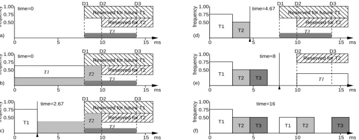
The final (and most aggressive) RT-DVS algorithm that we intro-duce in this paper attempts to achieve even better energy savings us-ing a look-ahead technique to determine future computation need and defer task execution. The cycle-conserving approaches dis-cussed above assume the worst case initially and execute at a high frequency until some tasks complete, and only then reduce operat-ing frequency and voltage. In contrast, the look-ahead scheme tries to defer as much work as possible, and sets the operating frequency to meet the minimum work that must be done now to ensure all future deadlines are met. Of course, this may require that we will be forced to run at high frequencies later in order to complete all of the deferred work in time. On the other hand, if tasks tend to use much less than their worst-case computing time allocations, the peak execution rates for deferred work may never be needed, and this heuristic will allow the system to continue operating at a low frequency and voltage while completing all tasks by their dead-lines.
Continuing with the example used earlier, we illustrate how a look-ahead RT-DVS EDF algorithm works in Figure 7. The goal is to defer work beyond the earliest deadline in the system (D1) so that
we can operate at a low frequency now. We allocate time in the schedule for the worst-case execution of each task, starting with the task with the latest deadline,T3. We spread outT3’s work
be-tweenD
1and its own deadline, D
3, subject to a constraint
reserv-ing capacity for future invocations of the other tasks (a). We repeat this step forT2, which cannot entirely fit betweenD1andD2after
allocatingT
3and reserving capacity for future invocations of T
1.
Additional work forT
2and all of T
1are allotted before D
1(b). We
note that more ofT2could be deferred beyondD1if we moved all
ofT3afterD2, but for simplicity, this is not considered. We use
the work allocated beforeD
1to determine the operating frequency.
OnceT1has completed, using less than its specified worst-case
ex-ecution cycles, we repeat this and find a lower operating frequency (c). Continuing this method of trying to defer work beyond the next deadline in the system ultimately results in the execution trace shown in (f).
select frequency(x):
use lowest freq.fi2ff1;:::;fmjf1<<fmg
such thatxf i
=f m
upon task release(Ti):
setcleft i
=C i;
defer();
upon task completion(T i):
setcleft i
= 0; defer();
during task execution(Ti):
decrementcleft i;
defer():
setU=C1=P1++Cn=Pn;
sets= 0;
fori= 1 ton, T i
2fT 1
;:::;T n
jD 1
D
n g
/* Note: reverse EDF order of tasks */ setU =U Ci=Pi;
setx= max(0,cleft i
(1 U)(D i
D n
));
setU =U+(cleft i
x)=(Di Dn);
sets=s+x;
select frequency (s=(D
n current time));
Figure 8: Look-Ahead DVS for EDF schedulers
The actual algorithm for look-ahead RT-DVS with EDF scheduling is shown in Figure 8. As in the cycle-conserving RT-DVS algorithm for RM, we keep track of the worst-case remaining computation
cleft
ifor the current invocation of task
Ti. This is set toCion task
release, decremented as the task executes, and set to 0 on comple-tion. The major step in this algorithm is the deferral funccomple-tion. Here, we look at the interval until the next task deadline, try to push as much work as we can beyond the deadline, and compute the mini-mum number of cycles,s, that we must execute during this interval
in order to meet all future deadlines. The operating frequency is set just fast enough to executescycles over this interval. To calculate s, we look at the tasks in reverse EDF order (i.e., latest deadline
first). Assuming worst-case utilization by tasks with earlier dead-lines (effectively reserving time for their future invocations), we calculate the minimum number of cycles,x, that the task must
exe-cute before the closest deadline,Dn, in order for it to complete by
its own deadline. A cumulative utilizationU is adjusted to reflect
the actual utilization of the task for the time afterD
n. This
cal-culation is repeated for all of the tasks, using assumed worst-case utilization values for earlier-deadline tasks and the computed val-ues for the later-deadline ones.sis simply the sum of thexvalues
calculated for all of the tasks, and therefore reflects the total num-ber of cycles that must execute byDnin order for all tasks to meet
their deadlines. Although this algorithm very aggressively reduces processor frequency and voltage, it ensures that there are sufficient cycles available for each task to meet its deadline after reserving worst-case requirements for higher-priority (earlier deadline) tasks.
2.6
Summary of RT-DVS algorithms
All of the RT-DVS algorithms we presented thus far should be fairly easy to incorporate into a real-time operating system, and do not require significant processing costs. The dynamic schemes all
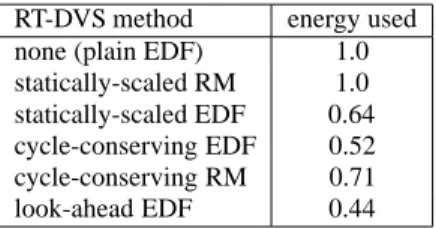
re-RT-DVS method energy used none (plain EDF) 1.0 statically-scaled RM 1.0 statically-scaled EDF 0.64 cycle-conserving EDF 0.52 cycle-conserving RM 0.71 look-ahead EDF 0.44
Table 4: Normalized energy consumption for the example traces
quireO(n)computation (assuming the scheduler provides an EDF
sorted task list), and should not require significant processing over the scheduler. The most significant overheads may come from the hardware voltage switching times. However, in all of our algo-rithms, no more than two switches can occur per task per invocation period, so these overheads can easily be accounted for, and added to, the worst-case task computation times.
To conclude our series of examples, Table 4 shows the normalized energy dissipated in the example task (Table 2) set for the first 16 ms, using the actual execution times from Table 3. We assume that the 0.5, 0.75 and 1.0 frequency settings need 3, 4, and 5 volts, respectively, and that idle cycles consume no energy. More general evaluation of our algorithms will be done in the next section.
3.
SIMULATIONS
We have developed a simulator to evaluate the potential energy sav-ings from voltage scaling in a real-time scheduled system. The following subsection describes our simulator and the assumptions made in its design. Later, we show some simulation results and provide insight into the most significant system parameters affect-ing RT-DVS energy savaffect-ings.
3.1
Simulation Methodology
Using C++, we developed a simulator for the operation of hardware capable of voltage and frequency scaling with real-time scheduling. The simulator takes as input a task set, specified with the period and computation requirements of each task, as well as several system parameters, and provides the energy consumption of the system for each of the algorithms we have developed. EDF and RM sched-ulers without any DVS support are also simulated for comparison.3
Parameters supplied to the simulator include the machine specifica-tion (a list of the frequencies and corresponding voltages available on the simulated platform) and a specification for the actual frac-tion of the worst-case execufrac-tion cycles that the tasks will require for each invocation. This latter parameter can be a constant (e.g., 0.9 indicates that each task will use 90% of its specified worst-case computation cycles during each invocation), or can be a random function (e.g., uniformly-distributed random multiplier for each in-vocation).
The simulation assumes that a constant amount of energy is re-quired for each cycle of operation at a given voltage. This quantum is scaled by the square of the operating voltage, consistent with en-ergy dissipation in CMOS circuits (E/V
2
). Only the energy con-sumed by the processor is computed, and variations due to
differ-3
Without DVS, energy consumption is the same for both EDF and RM, so EDF numbers alone would suffice. However, since some task sets are schedulable under EDF, but not under RM, we simulate both to verify that all task sets that are schedulable under RM are also schedulable when using the RM-based RT-DVS mechanisms.
ent types of instructions executed are not taken into account. With this simplification, the task execution modeling can be reduced to counting cycles of execution, and execution traces are not needed. The software-controlled halt feature, available on some processors and used for reducing energy expenditure during idle, is simulated by specifying an idle level parameter. This value gives the ratio be-tween energy consumed during a cycle while halted and that during a cycle of normal operation (e.g., a value of 0.5 indicates a cycle spent idling dissipates one half the energy of a cycle of compu-tation). For simplicity, only task execution and idle (halt) cycles are considered. In particular, this does not consider preemption and task switch overheads or the time required to switch operating frequency or voltages. There is no loss of generality from these simplifications. The preemption and task switch overheads are the same with or without DVS, so they have no effect on relative power dissipation. The voltage switching overheads incur a time penalty, which may affect the schedulability of some task sets, but incur al-most no energy costs, as the processor does not operate during the switching interval.
The real-time task sets are specified using a pair of numbers for each task, indicating its period and worst-case computation time. The task sets are generated randomly as follows. Each task has an equal probability of having a short (1–10ms), medium (10–100ms), or long (100–1000ms) period. Within each range, task periods are uniformly distributed. This simulates the varied mix of short and long period tasks commonly found in real-time systems. The com-putation requirements of the tasks are assigned randomly using a similar 3 range uniform distribution. Finally, the task computation requirements are scaled by a constant chosen such that the sum of the utilizations of the tasks in the task set reaches a desired value. This method of generating real-time task sets has been used previ-ously in the development and evaluation of a real-time embedded microkernel [31]. Averaged across hundreds of distinct task sets generated for several different total worst-case utilization values, the simulations provide a relationship of energy consumption to worst-case utilization of a task set.
3.2
Simulation Results
We have performed extensive simulations of the RT-DVS algo-rithms to determine the most important and interesting system pa-rameters that affect energy consumption. Unless specified other-wise, we assume a DVS-capable platform that provides 3 relative operating frequencies (0.5, 0.75, and 1.0) and corresponding volt-ages (3, 4, and 5, respectively).
In the following simulations, we compare our RT-DVS algorithms to each other and to a non-DVS system. We also include a theoret-ical lower bound for energy dissipation. This lower bound reflects execution throughput only, and does not consider any timing issues (e.g., whether any task is active or not). It is computed by taking the total number of task computation cycles in the simulation, and determining the absolute minimum energy with which these can be executed over the simulation time duration with the given platform frequency and voltage specification. No real algorithms can do bet-ter than this theoretical lower bound, but it is inbet-teresting to see how close our mechanisms approach this bound.
Number of tasks:
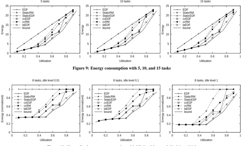
In our first set of simulations, we determine the effects of vary-ing the number of tasks in the task sets. Figure 9 shows the en-ergy consumption for task sets with 5, 10, and 15 tasks for all of our RT-DVS algorithms as well as unmodified EDF. All of these
simulations assume that the processor provides a perfect software-controlled halt function (so idling the processor will consume no energy), thus showing scheduling without any energy conserving features in the most favorable light. In addition, we assume that tasks do consume their worst-case computation requirements dur-ing each invocation. With these extremes, there is no difference be-tween the statically-scaled and cycle-conserving EDF algorithms. We notice immediately that the RT-DVS algorithms show poten-tial for large energy savings, particularly for task sets with mid-range worst-case processor utilization values. The look-ahead RT-DVS mechanism, in particular, seems able to follow the theoretical lower bound very closely. Although the total utilization greatly af-fects energy consumption, the number of tasks has very little effect. Neither the relative nor the absolute positions of the curves for the different algorithms shift significantly when the number of tasks is varied. Since varying the number of tasks has little effect, for all further simulations, we will use a single value.
Varying idle level:
The preceding simulations assumed that a perfect software-controlled halt feature is provided by the processor, so idle time consumes no energy. To see how an imperfect halt feature affects power con-sumption, we performed several simulations varying the idle level factor, which is the ratio of energy consumed in a cycle while the processor is halted, to the energy consumed in a normal execution cycle. Figure 10 shows the results for idle level factors 0.01, 0.1, and 1.0. Since the absolute energy consumed will obviously in-crease as the idle state energy consumption inin-creases, it is more insightful to look at the relative energy consumption by plotting the values normalized with respect to the unmodified EDF energy consumption.
The most significant result is that even with a perfect halt feature (i.e., idle level is 0), where the non-energy conserving schedulers are shown in the best light, there is still a very large percentage improvement with the RT-DVS algorithms. Obviously, as the idle level increases to 1 (same energy consumption as in normal oper-ation), the percentage savings with voltage scaling improves. The relative performance among the energy-aware schedulers is not sig-nificantly affected by changing the idle power consumption level, although the dynamic algorithms benefit more than the statically-scaled ones. This is evident as the cycle-conserving EDF mecha-nism results diverge from the statically-scaled EDF results. This is easily explained by the fact that the dynamic algorithms switch to the lowest frequency and voltage during idle, while the static ones do not; with perfect idle, this makes no difference, but as idle cycle energy consumption approaches that of execution cycles, the dy-namic algorithms perform relatively better. For the remainder of the simulations, we assume an idle level of 0.
Varying machine specifications:
All of the previous simulations used only one set of available fre-quency and voltage scaling settings. We now investigate the ef-fects of varying the simulated machine specifications. The follow-ing summarizes the hardware voltage and frequency settfollow-ings, where each tuple consists of the relative frequency and the corresponding processor voltage:
machine 0:f(0.5, 3), (0.75, 4), (1.0, 5)g
machine 1:f(0.5, 3), (0.75, 4), (0.83, 4.5), (1.0, 5)g
machine 2:f(0.36, 1.4), (0.55, 1.5), (0.64, 1.6),
0 5 10 15 20 25
0 0.2 0.4 0.6 0.8 1
Energy Utilization 5 tasks EDF StaticRM StaticEDF ccEDF ccRM laEDF bound 0 5 10 15 20 25
0 0.2 0.4 0.6 0.8 1
Energy Utilization 10 tasks EDF StaticRM StaticEDF ccEDF ccRM laEDF bound 0 5 10 15 20 25
0 0.2 0.4 0.6 0.8 1
Energy Utilization 15 tasks EDF StaticRM StaticEDF ccEDF ccRM laEDF bound
Figure 9: Energy consumption with 5, 10, and 15 tasks
0 0.2 0.4 0.6 0.8 1
0 0.2 0.4 0.6 0.8 1
Energy (normalized)
Utilization 8 tasks, idle level 0.01
EDF StaticRM StaticEDF ccEDF ccRM laEDF bound 0 0.2 0.4 0.6 0.8 1
0 0.2 0.4 0.6 0.8 1
Energy (normalized)
Utilization 8 tasks, idle level 0.1
EDF StaticRM StaticEDF ccEDF ccRM laEDF bound 0 0.2 0.4 0.6 0.8 1
0 0.2 0.4 0.6 0.8 1
Energy (normalized)
Utilization 8 tasks, idle level 1
EDF StaticRM StaticEDF ccEDF ccRM laEDF bound
Figure 10: Normalized energy consumption with idle level factors 0.01, 0.1, and 1.0
0 0.2 0.4 0.6 0.8 1
0 0.2 0.4 0.6 0.8 1
Energy (normalized)
Utilization 8 tasks, machine 0
EDF StaticRM StaticEDF ccEDF ccRM laEDF bound 0 0.2 0.4 0.6 0.8 1
0 0.2 0.4 0.6 0.8 1
Energy (normalized)
Utilization 8 tasks, machine 1
EDF StaticRM StaticEDF ccEDF ccRM laEDF bound 0 0.2 0.4 0.6 0.8 1
0 0.2 0.4 0.6 0.8 1
Energy (normalized)
Utilization 8 tasks, machine 2
EDF StaticRM StaticEDF ccEDF ccRM laEDF bound
Figure 11: Normalized energy consumption with machine 0, 1, and 2
0 0.2 0.4 0.6 0.8 1
0 0.2 0.4 0.6 0.8 1
Energy (normalized)
Utilization 8 tasks, c=0.9
EDF StaticRM StaticEDF ccEDF ccRM laEDF bound 0 0.2 0.4 0.6 0.8 1
0 0.2 0.4 0.6 0.8 1
Energy (normalized)
Utilization 8 tasks, c=0.7
EDF StaticRM StaticEDF ccEDF ccRM laEDF bound 0 0.2 0.4 0.6 0.8 1
0 0.2 0.4 0.6 0.8 1
Energy (normalized)
Utilization 8 tasks, c=0.5
EDF StaticRM StaticEDF ccEDF ccRM laEDF bound
0 0.2 0.4 0.6 0.8 1
0 0.2 0.4 0.6 0.8 1
Energy (normalized)
Utilization 8 tasks, uniform c
EDF StaticRM StaticEDF ccEDF ccRM laEDF bound
Figure 13: Normalized energy consumption with uniform dis-tribution for computation
Figure 11 shows the simulation results for machines 0, 1, and 2. Machine 0, used in all of the previous simulations, has frequency settings that can be expected on a standard PC motherboard, al-though the corresponding voltage levels were arbitrarily selected. Machine 1 differs from this in that it has the additional frequency setting, 0.83. With this small change, we expect only slight dif-ferences in the simulation results with these specifications. The most significant change is seen with cycle-conserving EDF (and statically-scaled EDF, since the two are identical here). With the extra operating point in the region near the cross-over point be-tween ccEDF and ccRM, the ccEDF algorithm benefits, shifting the cross-over point closer to full utilization.
Machine 2 is very different from the other two, and reflects the set-tings that may be available on a platform incorporating an AMD K6 processor with AMD’s PowerNow! mechanism [1]. Again, the voltage levels are only speculated here. As it has many more set-tings to select from, the plotted curves tend to be smoother. Also, since the relative voltage range is smaller with this specification, the maximum savings is not as good as with the other two machine specifications. More significant is the fact that the cycle-conserving EDF outperforms the look-ahead EDF algorithm. ccEDF and stat-icEDF benefit from the large number of settings, since this allows them to more closely match the task set and reduce energy ex-penditure. In fact, they very closely approximate the theoretical lower bound over the entire range of utilizations. On the other hand, laEDF sets the frequency trying to defer processing (which, in the worst case, would require running at full speed later). With more settings, the low frequency setting is closely matched, requir-ing high-voltage, high-frequency processrequir-ing later, hurtrequir-ing perform-ance. With fewer settings, the frequency selected would be some-what higher, so less processing is deferred, lessening the likelihood of needing higher voltage and frequency settings later, thus improv-ing performance. In a sense, the error due to a limited number of frequency steps is detrimental in the ccEDF scheme, but beneficial with laEDF. These results, therefore, indicate that the energy sav-ings from the various RT-DVS algorithms depend greatly on the available voltage and frequency settings of the platform.
Varying computation time:
In this set of experiments, we vary the distribution of the actual computation required by the tasks during each invocation to see how well the RT-DVS mechanisms take advantage of task sets that do not consume their worst-case computation times. In the
pre-ceding simulations, we assumed that the tasks always require their worst-case computation allocation. Figure 12 shows simulation re-sults for tasks that require a constant 90%, 70%, and 50% of their worst-case execution cycles for each invocation. We observe that the statically-scaled mechanisms are not affected, since they scale voltage and frequency based solely on the worst-case computation times specified for the tasks. The results for the cycle-conserving RM algorithm do not show significant change, indicating that it does not do a very good job of adapting to tasks that use less than their specified worst-case computation times. On the other hand, both the cycle-conserving and look-ahead EDF schemes show great reductions in relative energy consumption as the actual computa-tion performed decreases.
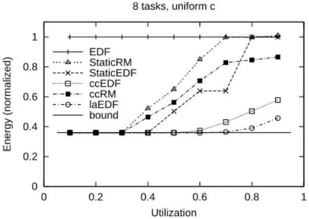
Figure 13 shows the simulation results using tasks with a uniform distribution between 0 and their worst-case computation. Despite the randomness introduced, the results appear identical to setting computation to a constant one half of the specified value for each invocation of a task. This makes sense, since the average execution with the uniform distribution is 0.5 times the worst-case for each task. From this, it seems that the actual distribution of computation per invocation is not the critical factor for energy conservation per-formance. Instead, for the dynamic mechanisms, it is the average utilization that determines relative energy consumption, while for the static scaling methods, the worst-case utilization is the deter-mining factor. The exception is the ccRM algorithm, which, albeit dynamic, has results that primarily reflect the worst-case utilization of the task set.
4.
IMPLEMENTATION
This section describes our implementation of a real-time scheduled system incorporating the proposed DVS algorithms. We will dis-cuss the architecture of the system and present measurements of the actual energy savings with our RT-DVS algorithms.
4.1
Hardware Platform
Although we developed the RT-DVS mechanisms primarily for em-bedded real-time devices, our prototype system is implemented on the PC architecture. The platform is a Hewlett-Packard N3350 notebook computer, which has an AMD K6-2+ [1] processor with a maximum operating frequency of 550 MHz. Some of the power consumption numbers measured on this laptop were shown earlier in Table 1. This processor features PowerNow!, AMD’s extensions that allow the processor’s clock frequency and voltage to be ad-justed dynamically under software control. We have also looked into a similar offering from Intel called SpeedStep [10], but this controls voltage and frequency through hardware external to the processor. Although it is possible to adjust the settings under soft-ware control, we were not able to determine the proper output se-quences needed to control the external hardware. We do not have experience with the Transmeta Crusoe processor [29] or with var-ious embedded processors (such as Intel XScale [9]) that are now supporting DVS.
The K6-2+ processor specification allows system software to se-lect one of eight different frequencies from its built-in PLL clock generator (200 to 600 MHz in 50 MHz increments, skipping 250), limited by the maximum processor clock rate (550 MHz here). The processor has 5 control pins that can be used to set the voltage through an external regulator. Although 32 settings are possible, there is only one that is explicitly specified (the default 2.0V set-ting); the rest are left up to the individual manufacturers. HP chose to incorporate only 2 voltage settings: 1.4V and 2.0V. The
volt-PowerNow Module
Periodic RT Task Module
RT Scheduler w/ RT−DVS
Scheduler Hook User
Kernel Level
Linux Kernel
RT Task Set DVS
Non−RT Level
Figure 14: Software architecture for RT-DVS implementation
age and frequency selectors are independently set, so we need a function to map each frequency to the appropriate available volt-age level. As there are no such specifications publicly available, we determined this experimentally. The processor was stable up to 450 MHz at 1.4 V, and needed the 2.0 V setting for higher frequen-cies. Stability was checked using a set of CPU-intensive bench-marks (mpg123in a loop and Linux kernel compile), and verifying proper behavior. We note that this empirical study used a sample size of one, so the actual frequency to voltage mappings may vary for other machines, even of the same model.
The processor has a mandatory stop interval associated with every change of the voltage or frequency transition, during which the pro-cessor halts execution. This mandatory halt duration is meant to en-sure that the voltage supply and clock have time to stabilize before the processor continues execution. As the characteristics of dif-ferent hardware implementations of the external voltage regulators can vary greatly, this stop duration is programmable in multiples of 41s (4096 cycles of the 100 MHz system bus clock). According
to our experience, it takes negligible time for frequency changes to occur. Using the CPU time-stamp register (basically a cycle counter), which continues to increment during the halt duration, we observed that around 8200 cycles occur during any transition to 200 MHz, and around 22500 cycles for a transition to 550 MHz, both with the minimum interval of 41s. This indicates that the
frequency of the CPU clock changes quickly and that most of the halt time is spent at the target frequency. We do not know the actual time required for voltage transition to occur, but in our experiments using a halt duration value of 10 (approximately 0.4 ms) resulted in no observable instability. The switching overheads in our system, therefore, are 0.4 ms when voltage changes, and 41s when only
frequency changes. As mentioned earlier, we can account for this switching overhead in the computation requirements of the tasks, since at most only two transitions are attributable to each task in each invocation.
4.2
Software Architecture
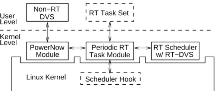
We implemented our algorithms as extension modules to the Linux 2.2.16 kernel. Although it is not a real-time operating system, Linux is easily extended through modules and provides a robust de-velopment environment familiar to us. The high-level view of our software architecture is shown in Figure 14. The approach taken for this implementation was to maximize flexibility and ease of use, rather than optimize for performance. As such, this implementation serves as a good proof-of-concept, rather than the ideal model. By implementing our kernel-level code as Linux kernel modules, we avoided any code changes to the Linux kernel, and these modules should be able to plug into unmodified 2.2.x kernels.
Digital Oscilloscope
Current Probe DC Adapter
(battery removed) Laptop
Figure 15: Power measurement on laptop implementation
The central module in our implementation provides support for pe-riodic real-time tasks in Linux. This is done by attaching call-back functions to hooks inside the Linux scheduler and timer tick han-dlers. This mechanism allows our modules to provide tight timing control as well as override the default Unix scheduling policy for our real-time tasks. Note that this module does not actually define the real-time scheduling policy or the DVS algorithm. Instead, we use separate modules that provide the real-time scheduling policy and the RT-DVS algorithms. One such RT scheduler/DVS module can be loaded on the system at a time. By separating the underly-ing periodic RT support from the schedulunderly-ing and DVS policies, this architecture allows dynamic switching of these latter policies with-out shutting down the system or the running RT tasks. (Of course, during the switch-over time between these policy modules, a real-time scheduler is not defined, and the real-timeliness constraints of any running RT tasks may not be met). The last kernel module in our implementation handles the access to the PowerNow! mechanism to adjust clock speed and voltage. This provides a clean, high-level interface for setting the appropriate bits of the processor’s special feature register for any desired frequency and voltage level. The modules provide an interface to user-level programs through the Linux/procfsfilesystem. Tasks can use ordinary file read and write mechanisms to interact with our modules. In particular, a task can write its required period and maximum computing bound to our module, and it will be made into a periodic real-time task that will be released periodically, scheduled according to the currently-loaded policy module, and will receive static priority over non-RT tasks on the system. The task also uses writes to indicate the com-pletion of each invocation, at which time it will be blocked until the next release time. As long as the task keeps the file handle open, it will be registered as a real-time task with our kernel extensions. Al-though this high-level, filesystem interface is not as efficient as di-rect system calls, it is convenient in this prototype implementation, since we can simply usecatto read from our modules and ob-tain status information in a human readable form. The PowerNow! module also provides a/procfsinterface. This will allow for a user-level, non-RT DVS demon, implementing algorithms found in other DVS literature, or to manually deal with operating frequency and voltage through simple Unix shell commands.
4.3
Measurements and Observations
We performed several experiments with our RT-DVS implementa-tion and measured the actual energy consumpimplementa-tion of the system. Figure 15 shows the setup used to measure energy consumption. The laptop battery is removed and the system is run using the ex-ternal DC power adapter. Using a special current probe, a digital oscilloscope is used to measure the power consumed by the lap-top as the product of the current and voltage supplied. This basic methodology is very similar to the one used in the PowerScope [6],
0 5 10 15 20 25 30
0 0.2 0.4 0.6 0.8 1
Power (Watts)
Utilization 5 tasks, real platform, c=0.9
EDF StaticRM ccEDF laEDF
Figure 16: Power consumption on actual platform
but instead of a slow digital multimeter, we use an oscilloscope that can show the transient behavior and also provide the true average power consumption over long intervals. Using the long duration acquisition capability of the digital oscilloscope, our power mea-surements are averaged over 15 to 30 second intervals.
Figure 16 shows the actual power consumption measured for our RT-DVS algorithms while varying worst-case CPU utilization for a set of 5 tasks which always consume 90% of their worst-case computation allocated for each invocation. The measurements re-flect the total system power, not just the CPU energy dissipation. As a result, there is a constant, irreducible power drain from the system board consumption (the display backlighting was turned off for these measurements; with this on, there would have been an additional constant 6 W to each measurement). Even with this overhead, our RT-DVS mechanisms show a significant 20% to 40% reduction in power consumption, while still providing the deadline guarantees of a real-time system.
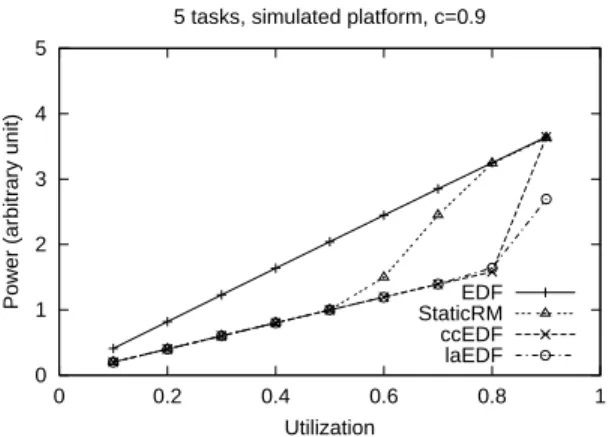
Figure 17 shows a simulation with identical parameters (including the 2 voltage-level machine specification) to these measurements. The simulation only reflects the processor’s energy consumption, so does not include any energy overheads from the rest of the sys-tem. It is clear that, except for the addition of constant overheads in the actual measurements, the results are nearly identical. This vali-dates our simulation results, showing that the results we have seen earlier really hold in real systems, despite the simplifying assump-tions in the simulator. The simulaassump-tions are accurate and may be useful for predicting the performance of RT-DVS implementations. We also note two interesting phenomena that should be consid-ered when implementing a system with RT-DVS. First, we noticed that the very first invocation of a task may overrun its specified computing time bound. This occurs only on the first invocation, and is caused by “cold” processor and operating system state. In particular, when the task begins execution, many cache misses, translation-look-aside buffer (TLB) misses, and page faults occur in the system (the last may be due to the copy-on-write page al-location mechanism used by Linux). These processing overheads count against the task’s execution time, and may cause it to exceed its bound. On subsequent invocations, the state is “warm,” and this problem disappears. This is due to the large difference between worst-case and average-case performance on general-purpose plat-forms, and explains why real-time systems tend to use specialized platforms to decrease or eliminate such variations in performance.
0 1 2 3 4 5
0 0.2 0.4 0.6 0.8 1
Power (arbitrary unit)
Utilization
5 tasks, simulated platform, c=0.9
EDF StaticRM ccEDF laEDF
Figure 17: Power consumption on simulated platform
The second important observation is that the dynamic addition of a task to the task set may cause transient missed deadlines unless one is very careful. Particularly with the more aggressive RT-DVS schemes, the system may be so closely matched to the current task set load that there may not be sufficient processor cycles remaining before the task deadlines to also handle the new task. One solution to this problem is to immediately insert the task into task set, so DVS decisions are based on the new system characteristics, but defer the initial release of the new task until the current invocations of all existing tasks have completed. This ensures that the effects of past DVS decisions, based on the old task set, will have expired by the time the new task is released.
5.
RELATED WORK
Recently, there have been a large number of publications describ-ing DVS techniques. Most of them present algorithms that are very loosely-coupled with the underlying OS scheduling and task man-agement systems, relying on average processor utilization to per-form voltage and frequency scaling [7, 23, 30]. They are basically matching the operating frequency to some weighted average of the current processor load (or conversely, idle time) using a simple feedback mechanism. Although these mechanisms result in close adaptation to the workload and large energy savings, they are un-suitable for real-time systems. More recent DVS research [4, 19] have shown methods of maintaining good interactive performance for general-purpose applications with voltage and frequency scal-ing. This is done through prediction of episodic interaction [4] or by applying soft deadlines and estimating task work distributions [19]. These methods show good results for maintaining short re-sponse times in human-interactive and multimedia applications, but are not intended for the stricter timeliness constraints of real-time systems.
Some DVS work has produced algorithms closely tied to the sched-uler [22, 24, 26], with some claiming real-time capability. These, however, take a very simplistic view of real-time tasks — only tak-ing into account a stak-ingle execution and deadline for a task. As such, they can only handle sporadic tasks that execute just once. They cannot handle the most important, canonical model of real-time systems, which uses periodic real-real-time tasks. Furthermore, it is not clear how new tasks entering the system can be handled in a timely manner, especially since all of the tasks are single-shot, and since the system may not have sufficient computing resources after having adapted so closely to the current task set.