Beyond the F Test:
Effect Size Confidence Intervals and Tests of Close Fit in the Analysis
of Variance and Contrast Analysis
James H. Steiger
Vanderbilt UniversityThis article presents confidence interval methods for improving on the standard F tests in the balanced, completely between-subjects, fixed-effects analysis of variance. Exact confidence intervals for omnibus effect size measures, such as2
and the root-mean-square standardized effect, provide all the information in the traditional hypothesis test and more. They allow one to test simultaneously whether overall effects are (a) zero (the traditional test), (b) trivial (do not exceed some small value), or (c) nontrivial (definitely exceed some minimal level). For situations in which single-degree-of-freedom contrasts are of primary interest, exact confi-dence interval methods for contrast effect size measures such as the contrast correlation are also provided.
The analysis of variance (ANOVA) remains one of the most commonly used methods of statistical analysis in the behavioral sciences. Most ANOVAs, especially in explor-atory studies, report an omnibus F test of the hypothesis that a main effect, interaction, or simple main effect is precisely zero. In recent years, a number of authors (Cohen, 1994; Rosnow & Rosenthal, 1996; Schmidt, 1996; Schmidt & Hunter, 1997; Serlin & Lapsley, 1993; Steiger & Fouladi, 1997) have sharply questioned the efficacy of tests of this “nil” hypothesis. Several of these critiques have concen-trated on ways that the nil hypothesis test fails to deliver the information that the typical behavioral scientist wants. However, a number of the articles have also suggested, more or less specifically, replacements for or extensions of the null hypothesis test that would deliver much more useful information.
The suggestions have developed along several closely related lines, including the following:
1. Eliminate the emphasis on omnibus tests, with
attention instead on focused contrasts that answer specific research questions, along with calculation of point estimates and approximate confidence
in-terval estimates for some correlational measures of effect size (e.g., Rosenthal, Rosnow, & Rubin, 2000; Rosnow & Rosenthal, 1996).
2. Calculate exact confidence interval estimates of
measures of standardized effect size, using an it-erative procedure (e.g., Smithson, 2001; Steiger & Fouladi, 1997).
3. Perform tests of a statistical null hypothesis other
than that of no difference or zero effect (e.g., Serlin & Lapsley, 1993).
As proponents of the first suggestion, Rosnow and Rosenthal (1996) discussed several types of correlation co-efficients that are useful in assessing experimental effects. Their work is particularly valuable in situations in which the researcher has questions that are best addressed by testing single contrasts. Rosnow and Rosenthal emphasized the use of the Pearson correlation, rather than the squared multiple correlation, partly because of concern that the latter tends to present an overly pessimistic picture of the value of “small” experimental effects.
The second suggestion, exact interval estimation, has been gathering momentum since around 1980. The move-ment to replace hypothesis tests with confidence intervals stems from the fundamental realization that, in many if not most situations, confidence intervals provide more of the information that the scientist is truly interested in. For example, in a two-group experiment, the scientist is more interested in knowing how large the difference between the two groups is (and how precisely it has been determined)
I express my gratitude to Michael W. Browne, Stanley A. Mulaik, the late Jacob Cohen, William W. Rozeboom, Rachel T. Fouladi, Gary H. McClelland, and numerous others who have encouraged this project.
Correspondence concerning this article should be addressed to James H. Steiger, Department of Psychology and Human Devel-opment, Box 512 Peabody College, Vanderbilt University, Nash-ville, TN 37203. E-mail: [email protected]
164 Note: This version includes corrections to the calculations at the bottom of page 173, Equation 51, and the discussion and confidence intervals on page 174, Table 3. Thanks to Professor Kris Kirby of Williams College for alerting me to these errors.
than whether the difference between the groups is exactly zero.
The third suggestion, which might be called tests of close
fit, has much in common with the approach widely known to
biostatisticians as bioequivalence testing and is based on the idea that the scientist should not be testing perfect adher-ence to a point hypothesis but should replace the test of close fit with a “relaxed” test of a more appropriate hypoth-esis. Tests of close fit share many of their computational aspects with the exact interval estimation approach in terms of the software routines required to compute probability levels, power, and sample size. They remain within the familiar hypothesis-testing framework, while providing im-portant practical and conceptual gains, especially when the experimenter’s goal is to demonstrate that an effect is trivial.
In this article, I present methods that implement; support; and, in some cases, unify and extend major suggestions (1) through (3) discussed above. First I briefly review the his-tory, rationale, and theory behind exact confidence intervals on measures of standardized effect size in ANOVA. I then provide detailed instructions, with examples, and software support for computing these confidence intervals. Next I discuss a general procedure for assessing effects that are represented by one or more contrasts, using correlations. Included is a population rationale, with sampling theory and an exact confidence interval estimation procedure, for one of the correlational measures discussed by Rosnow and Rosenthal (1996).
Although the initial emphasis is on confidence interval estimation, I also discuss how the same technology that generates confidence intervals may be used to test hypoth-eses of minimal effect, thus implementing the good enough
principle discussed by Serlin and Lapsley (1993).
Exact Confidence Intervals on Standardized Effect Size
The notion that hypothesis tests of zero effect should be replaced with exact confidence intervals on measures of effect size has been around for quite some time but was somewhat impractical because of its computational de-mands until about 10 years ago. A general method for constructing the confidence intervals, which Steiger and Fouladi (1997) referred to as noncentrality interval
estima-tion, is considered elementary by statisticians but seldom is
discussed in behavioral statistics texts. In this section, I review some history, then describe the method of noncen-trality interval estimation in detail.
Rationale and History
Suppose that, as a researcher, you test a drug that you believe enhances performance. You perform a simple
two-group experiment with a double-blind control. In this case, you are engaging in “reject–support” (R-S) hypothesis test-ing (rejecttest-ing the null hypothesis will support your belief). The null and alternative hypotheses might be
H0:1ⱕ2; H1:1⬎2. (1)
The null hypothesis states that the drug is no better than a placebo. The alternative, which the investigator believes, is that the drug enhances performance. Rejecting the null hypothesis, even at a very low alpha such as .001, need not indicate that the drug has a strong effect, because if sample size is very large relative to the sampling variability of the drug effect, even a trivial effect might be declared highly significant. On the other hand, if sample size is too low, even a strong effect might have a low probability of creating a statistically significant result.
Statistical power analysis (Cohen, 1988) and sample size estimation have been based on the notion that calculations made before data are gathered can help to create a situation in which neither of the above problems is likely to occur. That is, sample size is chosen so that power will be high, but not too high.
There is an alternative situation, “accept–support” (A-S) testing, that attracts far less attention than R-S testing in statistics texts and has had far less impact on the popular wisdom of hypothesis testing. In A-S testing, the statistical null hypothesis is what the experimenter actually wishes to prove. Accepting the statistical null hypothesis supports the researcher’s theory. Suppose, for example, an experiment provides convincing evidence that the above-mentioned drug actually works. The next step might be to provide convincing evidence that it has few, or acceptably low, side effects.
In this case two groups are studied, and some measure of side effects is taken. The null hypothesis is that the exper-imental group’s level of side effects is less than or equal to the control group’s level. The researcher (or drug company) supporting the research wants not to reject this null hypoth-esis, because in this case accepting the null hypothesis supports the researcher’s point of view, that is, that the drug is no more harmful than its predecessors.
In a similar vein, a company might wish to show that a generic drug does not differ appreciably in bioavailability from its brand name equivalent. This problem of bioequiva-lence testing is well known to biostatisticians and has re-sulted in a very substantial literature (e.g., Chow & Liu, 2000).
Suppose that Drug A has a well-established
bioavailabil-ity levelA, and an investigator wishes to assess the
bio-equivalence of Drug B with Drug A. One might engage in A-S testing, that is, test the null hypothesis that
and declare the two drugs bioequivalent if this null hypoth-esis is not rejected. However, the perils of such A-S testing are even greater than in R-S testing. Specifically, simply running a sloppy, low-power experiment will tend to result in nonrejection of the null hypothesis, even if the drugs differ appreciably in bioavailability. Thus, paradoxically, someone trying to establish the bioequivalence of Drug B with Drug A could virtually guarantee success simply by using too small a sample size. Moreover, with extremely large sample sizes, Drug B might be declared nonequivalent to Drug A even if the difference between them is trivial.
Because of such problems, biostatisticians decided long ago that the test for strict equality is inappropriate for bioavailability studies (Metzler, 1974). Rather, a dual hy-pothesis test should be performed. Suppose that the Food and Drug Administration has determined that any drug with
bioavailability within 20% of A may be considered
bio-equivalent and prescribed in its stead. Suppose that1and
2represent these bioequivalence limits. Then establishing
bioequivalence of Drug B with Drug A might amount to rejecting the following hypothesis,
H0:B⬎2orB⬍1 (3)
against the alternative
Ha:1ⱕBⱕ2. (4)
In practice, this usually amounts to testing two one-sided hypotheses,
H01:Bⱕ1versus Ha1:B⬎1 (5)
and
H02:Bⱖ2versus Ha2:B⬍2. (6)
An alternative approach (Westlake, 1976) is to construct
a confidence interval forB. Bioequivalence would be
de-clared if the confidence interval falls entirely within the established bioequivalence limits.
In other contexts, particularly the more exploratory stud-ies performed in psychology, the research goal may be simply to pinpoint the nature of a parameter rather than to decide whether it is within a known fixed range. In that case, reporting the endpoints of a confidence interval (without announcing an associated decision) may be an appropriate conclusion to an analysis. In any case, because the hypoth-esis test may be performed with the confidence interval, it seems that the confidence interval should always be re-ported. It contains all the information in a hypothesis test result, and more.
In structural equation modeling, which includes factor analysis and multiple regression as special cases, statistical testing prior to 1980 was limited to a chi-square test of perfect fit. In this procedure, the statistical null hypothesis is
that the model fits perfectly in the population. This hypoth-esis test was performed, and a model was judged to fit the data “sufficiently well” if the null hypothesis was not re-jected. There was widespread dissatisfaction with the test, because no model would be expected to fit perfectly, and so large sample sizes usually led to rejection of a model, even if it fit the data quite well. In this arrangement, enhanced precision actually worked against the researcher’s interests. Steiger and Lind (1980) suggested that the traditional null hypothesis test of perfect fit of a structural model be re-placed by a confidence interval on the root-mean-square error of approximation (RMSEA), an index of population badness of fit that compensated for the complexity of the model.
MacCallum, Browne, and Sugawara (1996) suggested augmenting the confidence interval with a pair of hypothesis tests. They considered a population RMSEA value of .05 to be indicative of a close-fitting model, whereas a value of .08 or more was evidence of marginal to poor fit. Consequently, a test of close fit would test the null hypothesis that the RMSEA is greater than or equal to .05 against the alterna-tive that it is less than .05. Rejection of the null hypothesis indicates close fit. A test of not-close fit tests the null hypothesis that the RMSEA is less than or equal to .08 against the alternative that it is greater than .08. Rejection of the null hypothesis indicates that fit is not close. MacCallum et al. demonstrated in detail how, with such hypothesis tests, power calculations could be performed and required sample sizes estimated. These two one-sided tests can be performed
easily and simultaneously with a single 1⫺2␣confidence
interval recommended by Steiger (1989). Simply construct the confidence interval and see whether its upper end is below .05 (in which case the test of close fit results in rejection at the alpha level) and whether its lower end exceeds .08 (in which case the test of not-close fit results in rejection at the alpha level). The confidence interval pro-vides all the information in both hypothesis tests, and more. Fleishman (1980) suggested interval estimation as a sup-plement for the F test in ANOVA. He gave examples of how to compute exact confidence intervals on a number of useful quantities, such as the signal-to-noise ratio, in ANOVA. These confidence intervals offered clear advan-tages over the traditional hypothesis test. Other authors have noted the existence of exact confidence intervals for the standardized effect size in the simplest special case of ANOVA, the two-sample t test (e.g., Hedges & Olkin, 1985).
The rationale for switching from hypothesis testing to confidence interval estimation is straightforward (Steiger & Fouladi, 1997). Unfortunately, the exact interval estimation procedures of Steiger and Lind (1980), Fleishman (1980), and Hedges and Olkin (1985) are virtually impossible to compute accurately by hand. However, by 1990, microcom-puter capabilities had advanced substantially. The RMSEA
confidence interval was implemented in general purpose structural equation modeling software (Mels, 1989; Steiger, 1989) and, by the late 1990s, had achieved widespread use. Steiger (1990) presented general procedures for construct-ing confidence intervals on measures of effect size in co-variance structure analysis, ANOVA, contrast analysis, and multiple regression. Steiger and Fouladi (1992) produced a general computer program, R2, that performed exact confi-dence interval estimation of the squared multiple correlation in multiple regression. Taylor and Muller (1995, 1996) have presented general procedures for analyzing power and non-centrality in the general linear model, including an analysis of the impact of restriction of published articles to signifi-cant results. Steiger and Fouladi (1997) demonstrated gen-eral procedures for confidence interval calculations, and Steiger (1999) implemented these in a commercial software package. Smithson (2001) discussed a number of confi-dence interval procedures in fixed and random regression models and included SPSS macros for calculating confi-dence intervals for noncentral distributions. Reiser (2001) discussed confidence intervals on functions of Mahalanobis distance.
General Theory of Noncentrality-Based Interval Estimation
In this section, I review the general theoretical principles for constructing exact confidence intervals for effect size, power, and sample size in the balanced fixed-effects be-tween-subjects ANOVA. For a more detailed discussion of these principles, see Steiger and Fouladi (1997). Through-out what follows, I adopt a simple notational device: When
several groups or cells are sampled, I use Ntotto stand for
the total sample size and use n to stand for the number of observations in each group.
I begin this section with a brief nontechnical discussion of noncentral distributions. The t, chi-square, and F distribu-tions are special cases of more general distribudistribu-tions called the noncentral t, noncentral chi-square, and noncentral F. Each of these noncentral distributions has an additional parameter, called the noncentrality parameter. For example, whereas the F distribution has two parameters (the numer-ator and denominnumer-ator degrees of freedom), the noncentral F has these two plus a noncentrality parameter (often
indi-cated with the symbol). When the noncentral F
distribu-tion has a noncentrality parameter of zero, it is identical to the F distribution, so it includes the F distribution as a special case. Similar facts hold for the t and chi-square distributions. What makes the noncentrality parameter es-pecially important is that it is related very closely to the truth or falsity of the null hypotheses that these distributions are typically used to test. Thus, for example, when the null hypothesis of no difference between two means is correct, the standard t statistic has a distribution that has a
noncen-trality parameter of zero, whereas if the null hypothesis is false, it has a noncentral t distribution, that is, the noncen-trality parameter is nonzero. The more false the null hy-pothesis, the larger the absolute value of the noncentrality parameter for a given alpha and sample size.
Most confidence intervals in introductory textbooks are derived by simple manipulation of a statement about inter-val probability of a sampling distribution. This approach cannot be used to generate exact confidence intervals for many quantities of fundamental importance in statistics. As an example, consider the sample squared multiple correla-tion, whose distribution changes as a function of the popu-lation squared multiple correpopu-lation. Confidence intervals for the squared multiple correlation are very informative yet are not discussed in standard texts, because a single simple formula for the direct calculation of such an interval cannot be obtained in a manner analogous to the way one obtains a
confidence interval for the population mean. Steiger and
Fouladi (1997) discussed a general method for confidence interval construction that handles many such interesting examples. The method combines two general principles, which they called the confidence interval transformation
principle and the inversion confidence interval principle.
The former is obvious but seldom discussed formally. The latter is referred to by a variety of names in textbooks and review articles (Casella & Berger, 2002; Steiger & Fouladi, 1997), yet it does not seem to have found its way into the standard behavioral statistics textbooks, primarily because its implementation involves some difficult computations. However, the method is easy to discuss in principle and is no longer impractical. When the two principles are com-bined, a number of very useful confidence intervals result.
Proposition 1: Confidence interval transformation prin-ciple. Let f() be a monotone function of , that is, a function whose slope never changes sign and is never zero.
Let l1 and l2 be lower and upper endpoints of a 1 ⫺ ␣
confidence interval on quantity. Then, if the function is
increasing, f(l1) and f(l2) are lower and upper endpoints,
respectively, of a 100(1⫺␣)% confidence interval on f().
If the function is decreasing, f(l2) and f(l1) are lower and
upper endpoints. Here are two elementary examples of this principle.
Example 1: Suppose you read in a textbook how to
calculate a confidence interval for the population variance
2
. However, you desire a confidence interval for .
Be-causetakes on only nonnegative values, it is a monotonic
increasing function of2over its domain. Hence, the
con-fidence interval foris obtained by taking the square root
of the endpoints for the corresponding confidence interval for2.
Example 2: Suppose one calculates a confidence interval
for z(), the Fisher transform of, the population correlation coefficient. Taking the inverse Fisher transform of the end-points of this interval will give a confidence interval for.
This is, in fact, the method used to calculate the standard confidence interval for a correlation.
These examples show why Proposition 1 is very useful in practice. A statistical quantity we are very interested in—
such as—may be a simple function of a quantity—such as
z()—we are not so interested in, but for which we can
easily obtain a confidence interval. Next, we define the inversion confidence interval principle.
Proposition 2: Inversion confidence interval principle.
Let x be the observed value of X, a random variable with a
continuous cdf (cumulative distribution function) F(x,)⫽
Pr(X ⱕ x兩) for some numerical parameter . Let ␣1 ⫹
␣2⫽␣with 0⬍␣⬍1 be fixed values. If F(x,) is strictly
decreasing in, for fixed values of x, choose l1(x) and l2(x)
so that Pr[Xⱕ x兩 ⫽l1(x)]⫽ 1⫺␣2and Pr[X ⱕx兩 ⫽
l2(x)]⫽ ␣1. If F(x, ) is strictly increasing in, for fixed
values of x, choose l1(x) and l2(x) so that Pr[Xⱕx兩⫽l1(x)]
⫽␣1and Pr[Xⱕx兩⫽l2(x)]⫽1⫺␣2. Then the random
interval [l1(x), l2(x)] is a 100(1⫺ ␣)% confidence interval
for. Upper or lower 100(1⫺␣)% confidence bounds (or
“one-sided confidence intervals”) may be obtained by set-ting␣1or␣2to zero.
For a simple graphically based explanation of Proposition 2, consult Steiger and Fouladi (1997, pp. 237–239). For a clear, succinct discussion with partial proof, see Casella and Berger (2002, p. 432), who referred to this as “pivoting” the
cdf. In this article, I assume␣1⫽␣2⫽␣/2, although such
an interval may not be the minimum width for a given␣.
Proposition 2 implies a simple approach to interval estima-tion: Suppose you have observed an F statistic with a value
x and known degrees of freedom 1 and 2. Denote the
cumulative distribution of the F statistic by F(x,), where is the noncentrality parameter. It can be shown that if1,2,
and x are held constant at any positive value, then F(x,) is
strictly decreasing in. Accordingly, Proposition 2 can be
used. To calculate a 100(1⫺␣)% confidence interval on the
noncentrality parameter of the F distribution, use the fol-lowing steps.
1. Calculate the cumulative probability p of x in the
central F distribution. If p is below␣/2, then both limits of the confidence interval are zero. If p is
below 1⫺ ␣/2, the lower limit of the confidence
interval is zero, and the upper limit must be cal-culated (go to Step 3). Otherwise, calculate both limits of the confidence interval, using Steps 2 and 3.
2. To calculate the lower limit, find the unique value
of that places x at the 1 ⫺ ␣/2 cumulative
probability point of a noncentral F distribution
with1and2degrees of freedom.
3. To calculate the upper limit, find the unique value
ofthat places x at the␣/2 cumulative probability point of a noncentral F distribution with1and2
degrees of freedom.
Calculating a confidence interval forthus requires
iter-ative calculation of the unique value of that places an
observed value of F at a particular percentile of the
non-central F distribution.1In what follows, I give a variety of
examples of confidence interval calculations. Some will be at the 95% level of confidence, others at the less common 90% level. In a later section, I discuss why, when confi-dence intervals are used to perform a hypothesis test at the .05 level, a 90% interval may be appropriate in some situ-ations and a 95% interval in others. At that point, I describe how to select confidence intervals at the appropriate level to perform a particular hypothesis test.
Measures of Standardized Effect Size
Now I examine some more ambitious examples. For simplicity of exposition, I assume in this section that either the freeware program NDC (noncentral distribution calcu-lator; see Footnote 1) or other software is available to
compute a confidence interval on, the noncentrality
pa-rameter of a noncentral F distribution. Consider the one-way, fixed-effects ANOVA, in which p means are compared for equality, and there are n observations per group. The overall F statistic has a distribution that is a noncentral F,
with degrees of freedom p⫺1 and p(n ⫺1) ⫽Ntot⫺p.
The noncentrality parameter can be expressed in a
number of ways. One formula that appears frequently in textbooks is
⫽n
冘
j⫽1
p
冉
␣j
冊
2. (7)
The␣jvalues in Equation 7 are the effects as commonly
defined in ANOVA, that is,
␣j⫽j⫺. (8)
If j is the mean of the jth group, and is the overall
mean, thenis, in the case of equal n, simply the arithmetic
average of thej. More generally (although in what follows
I assume a balanced design unless stated otherwise),
⫽
冘
j⫽1
p
nj
Ntot
j. (9)
1
NDC (noncentral distribution calculator), a freeware Windows program for calculating percentage points and noncentrality con-fidence intervals for noncentral F, t, and chi-square distributions, is available for direct download from the author’s website (http:// www.statpower.net).
The quantity ␣j/ is a standardized effect, that is, the effect expressed in standard deviation units. The quantity
/n is therefore the sum of squared standardized effects.
There are numerous ways one might convert the sum of squared standardized effects into an overall measure of effect size. For example, suppose we average these squared standardized effects in order to obtain an overall measure of strength of effects in the design. The arithmetic average of the p squared standardized effects, sometimes called the
signal-to-noise ratio (Fleishman, 1980), is as follows:
f2⫽1
p
冘
j⫽1
p
冉
␣j
冊
2⫽np ⫽N tot
. (10)
One problem with this measure is that it is the average squared effect and so is not in the proper unit of measure-ment. A potential solution is to simply take the square root of the signal-to-noise ratio, obtaining
f⫽
冑
Ntot⫽冑
1
p
冘
j⫽1
p
冉
␣j
冊
2. (11)
In a one-way ANOVA with p groups and equal n, the effects are constrained to sum to zero, so there are actually
only p⫺ 1 independent effects. Thus, an alternative
mea-sure, /[(p ⫺ 1)n], is the average squared independent
standardized effect, and the root-mean-square standardized effect (RMSSE) is as follows:
⌿⫽
冑
共p⫺1兲n⫽冑
p⫺11冘
j⫽1
p
冉
␣j
冊
2. (12)
Equations 11 and 12 demonstrate that the relationships
between ⌿, f, and the noncentrality parameter are
straightforward.
In order to obtain a confidence interval for⌿, we proceed
as follows. First, we obtain a confidence interval estimate
for. Next, we invoke the confidence interval
transforma-tion principle to directly transform the endpoints by
divid-ing by (p⫺1)n. Finally, we take the square root. The result
is an exact confidence interval on⌿.
Example 3: Suppose a one-way fixed-effects ANOVA is
performed on four groups, each with a sample size of 20, and that an overall F statistic of 5.00 is obtained, with 3 and 76 degrees of freedom, with a probability level of .0032. The F test is thus “highly significant,” and the null hypoth-esis is rejected at the .01 level. Some investigators might interpret this result as implying that a powerful experimen-tal effect was found and that this was determined with high precision. In this case, the noncentrality interval estimate provides a more informative and somewhat different ac-count of what has been found.
The 95% confidence interval forranges from 1.8666 to
32.5631. To convert this to a confidence interval for⌿, we
use Equation 12. The corresponding confidence interval for
⌿ranges from .1764 to .7367. Effects are almost certainly
“here,” but they are on the order of half a standard devia-tion, what is commonly considered a medium-size effect. Moreover, the size of the effects has not been determined with high precision.
Example 4: Fleishman (1980) described the calculation of
confidence intervals on the noncentrality parameter of the noncentral F distribution to obtain, in a manner equivalent to that used in the previous two examples, confidence in-tervals on f2and2, the latter of which is defined as
A(partialed)
2 ⫽ SA
2
SA
2 ⫹ e
2, (13)
where S
A
2 is the variance of p means for the levels of a
particular effect A, that is,
SA
2 ⫽共
1/p兲
冘
j⫽1
p
共j⫺兲2 (14)
and e
2
is the within-cell variance. A(partialed) 2
may be thought of as the proportion of the variance remaining (after all other main effects and interactions have been partialed out) that is explained by the effect. (In what follows, for simplicity, I refer to the coefficient simply as2.) There are simple relationships between f2,2, and, specifically,
f2⫽ 2
1⫺2⫽
pn⫽
Ntot
(15) and
2⫽ f 2
1⫹f2⫽
⫹Ntot
. (16)
Fleishman (1980) cited an example given by Venables
(1975) of a five-group ANOVA with n⫽11 per cell and an
observed F of 11.221. In this case the 90% confidence
interval for the noncentrality parameter has endpoints
19.380 and 71.549. Once we obtain the confidence interval
for , it is a trivial matter to transform the limits of the
interval to confidence limits for2, using Equation 16. For
example, the lower limit becomes 19.380
19.380⫹共5兲共11兲⫽
19.380
19.380⫹55⫽
19.380
74.380⫽.261.
(17) In a similar manner, the upper limit of the confidence interval can be calculated as .565. The confidence interval has determined with 90% confidence that the main effect
accounts for between 26.1% and 56.5% of the variance in the dependent variable.
General Procedures for Effect Size Intervals in Between-Subjects Factorial ANOVA
In a previous example, we saw how easy it is to construct a confidence interval on measures of effect size in one-way
ANOVA, provided a confidence interval for has been
computed. In this section, a completely general method is demonstrated for computing confidence intervals for vari-ous measures of standardized effect size in completely between-subjects factorial ANOVA designs with equal sample size n per cell.
We begin with a general formula relating the
noncentral-ity parameter with the RMSSE in any completely
be-tween-subjects factorial ANOVA. Letstand for a
partic-ular effect, and n the sample size per cell. Then
⌿⫽
冑
ndf. (18)
In Equation 18, nis equal to n (the number of observations in each cell of the design) multiplied by the product of the numbers of levels in all the factors not represented in the effect currently under consideration; dfis the numerator degrees of freedom parameter for the effect under consideration.
There are simple relationships between the RMSSE and other measures of standardized effect size. Specifically, for a general factorial ANOVA,
f2⫽
⌿2df
Cells⫽
Ntot
, (19)
where Cellsis, for any main effect, the number of levels of
the effect. For any interaction, it is the product of the numbers of levels for all factors involved in the interaction.
The relationship between f2and2is given in Equation 16.
Some examples of these quantities, for a four-way ANOVA, with p, q, r, and s levels of factors A, B, C, and D, respectively, are given in Table 1. The table may be used also for one-, two-, or three-way ANOVAs simply by elim-inating terms involving levels not represented in the design. For example, in a three-way ANOVA, the BC interaction
effect has (q⫺1)(r⫺1) numerator degrees of freedom, and
nBC is np, because there is no s in this design. The error
degrees of freedom in a three-way ANOVA are pqr(n⫺1).
In the following two examples, I demonstrate how to com-pute a 90% confidence interval on various measures of effect, using the information in the table.
Example 5: Suppose that, as a researcher, you perform a
three-way 2⫻3⫻7 ANOVA, with n⫽6 observations per
cell. In this case, we have p⫽2, q⫽ 3, and r⫽ 7.
Suppose that, for the A main effect, you observe an F statistic of 4.2708, which, with 1 and 210 degrees of
free-dom, has p⫽.0400. We first calculate a confidence interval
for. The endpoints of this interval arelower⫽0.100597
andupper⫽13.8186. To convert these to confidence
inter-vals on⌿, f2, f, and2, we apply Equations 18, 19, and 16.
For the A effect, we have nA⫽(6)(3)(7)⫽126, dfA⫽(2⫺
1)⫽1, CellsA⫽2, and Ntot⫽252. Hence, for⌿we have,
from Equation 18,
⌿lower⫽
冑
0.100597
共126兲共1兲 ⫽0.028256,⌿upper
⫽
冑
共13.8186126兲共1兲⫽0.331167. (20)For f2and f we have, for the lower limits,
flower
2 ⫽0.100597
252 ⫽0.000399194, flower⫽0.01998. (21)
For the upper limits, we obtain fupper2 ⫽ 0.0548357 and
fupper⫽ 0.234170.
We can also convert the confidence limits for f2 into
limits for2, using Equation 16. We have
lower
2 ⫽ flower 2
1⫹flower
2 ⫽
0.000399194
1.000399194⫽0.000399035. (22)
In a similar manner, we obtain the upper limit asupper2 ⫽
0.0519851.
Example 6: Table 1 can also be used for a two-way
ANOVA, simply by letting r⫽1 and s⫽1 and ignoring all
Table 1
Key Quantities for Computing Effect Size Intervals in Four-Way Analysis of Variance
Source Levels df n
A p p⫺1 nqrs
B q q⫺1 nprs
C r r⫺1 npqs
D s s⫺1 npqr
AB (p⫺1)(q⫺1) nrs
AC (p⫺1)(r⫺1) nqs
AD (p⫺1)(s⫺1) nqr
BC (q⫺1)(r⫺1) nps
BD (q⫺1)(s⫺1) npr
CD (r⫺1)(s⫺1) npq
ABC (p⫺1)(q⫺1)(r⫺1) ns
ABD (p⫺1)(q⫺1)(s⫺1) nr
ACD (p⫺1)(r⫺1)(s⫺1) nq
BCD (q⫺1)(r⫺1)(s⫺1) np
ABCD (p⫺1)(q⫺1)(r⫺1)(s⫺1) n
Error pqrs(n⫺1)
Note. represents a particular effect; n represents the sample size per cell; and p, q, r, and s represent levels of factors A, B, C, and D, respectively.
effects involving factors C and D. Suppose, for example,
one were to perform a two-way 2⫻7 ANOVA, with n⫽
4 observations per cell, and the F statistic for the AB interaction is observed to be 2.50. The key quantities are dfAB
⫽6, dferror⫽ 42, nAB⫽ 4, and CellsAB⫽ 14. The
confi-dence limits forABare lower ⫽ 0.462800 and upper ⫽
25.8689. Consequently, from Equation 18, the confidence limits for the RMSSE are
⌿lower⫽
冑
lowernABdfAB⫽
冑
0.462800
共4兲共6兲 ⫽0.1389, (23)
⌿upper⫽
冑
25.8689
共4兲共6兲 ⫽1.0382. (24)
The confidence intervals for f2and f are
flower
2 ⫽0.462800
56 ⫽0.008264, flower⫽0.0909, (25)
fupper
2 ⫽25.8689
56 ⫽0.461944, fupper⫽0.6797. (26)
Using Equation 16, we convert the above to the following confidence limits for2:
lower
2 ⫽ flower 2
1⫹flower
2 ⫽
0.008264
1.008264⫽0.0082, (27)
upper
2 ⫽0.461944
1.461944⫽0.3160. (28)
Multiple Regression With Fixed Regressors
One standardized index of the size of effects is to com-pute the squared multiple correlation coefficient between the independent variable and the scores on the dependent variable. This index, in the population, characterizes the strength of the effect. ANOVA may be conceptualized as a linear regression model with fixed independent variables. In this case, the theory of multiple regression with fixed re-gressors applies. It is important to realize (e.g., Sampson, 1974) that the theory for fixed regressors, although it shares many similarities with that for random regressors, has im-portant differences, which are especially apparent when considering the nonnull distributions of the variables. The general model is
E共兲⫽X, (29)
where is an Ntot ⫻ 1 random vector, X is an Ntot ⫻ p
matrix, andis a p⫻ 1 vector of unknown parameters.
This model includes model errors (⑀) that are assumed to
be independently and identically distributed with a normal distribution, zero mean, and variance2. That is,
⫽X⫹⑀⫽ˆ ⫹⑀, (30)
and⑀has a multivariate normal distribution with zero mean
vector 0 and covariance matrix 2I, with I an identity
matrix. It is common to partitioninto
⫽
冋
01
册
, (31)where0is an intercept term. Correspondingly, X is
parti-tioned as
X⫽关1 X1兴, (32)
where 1 is a column of ones and X1contains the original X
scores transformed into deviations about their sample means.
Consider now a set of observed scores y, representing
realizations of the random variables in. If X1has p⫺ 1
columns, then an F statistic for testing the hypothesis that
1⫽ 0 is
F⫽ R
2
/共p⫺1兲
共1⫺R2兲
/共Ntot⫺p兲
. (33)
This statistic has a noncentral F distribution with p⫺1 and
Ntot⫺p degrees of freedom, with a noncentrality parameter
given by
⫽⬘X⬘共I⫺P1兲X
2 ⫽
⬘X⬘Q1X
2 . (34)
For any matrix A of full column rank, PA is the column
space projection operator A(A⬘A)⫺1A⬘and QAthe
comple-mentary projector I⫺PA.
We now turn to an application of this theory in the context of ANOVA. Consider the simple case of a one-way fixed-effects ANOVA with n observations in each of p independent groups. It is well-known that this model can be written in the form of Equation 29, where X is a design
matrix with Ntot⫽np rows and p columns, andcontains
ANOVA parameters.
We are not interested in R2per se. Rather, we are
inter-ested in the corresponding quantity2in an infinite
popu-lation of observations in which treatment groups are repre-sented equally. There are several alternative ways of
conceptualizing such a quantity. Formally, we can define2
as the probability limit of R2, that is,
2⫽
plim n3⬁共
R2兲
. (35)
This is the constant that R2converges to as the sample size
increases without bound. It can be proven (see Appendix A) that, with this definition of2, the noncentrality parameter is
⫽Ntot 2
1⫺2, (36)
and so
2⫽
⫹Ntot
. (37)
Consequently, a confidence interval formay be converted
easily into a confidence interval on 2or , because is
nonnegative.2represents the coefficient of determination
for predicting scores on the dependent variable from only a knowledge of the population means of the groups in an infinite population in which all treatment groups are equally represented.
Example 7: Suppose that X is set up as in Equation 38 to
represent a full rank design matrix for a one-way ANOVA,
with three groups, and n⫽3, and that the scores in y are 1,
2, 3, 4, 5, 6, 7, 8, 9. In this parameterization,0corresponds
to3, 1corresponds to 1⫺ 3, and2 corresponds to
2 ⫺ 3. The group means are 2, 5, 8, and the group
variances are all 1.
冤
y11y21
y31
y12
y22
y32
y13
y23
y33
冥
⫽冤
1 1 0
1 1 0
1 1 0
1 0 1
1 0 1
1 0 1
1 0 0
1 0 0
1 0 0
冥
冋
01 2
册
⫹
冤
⑀11 ⑀21 ⑀31 ⑀12 ⑀22 ⑀32 ⑀13 ⑀23 ⑀33冥
. (38)
In this case, it is easy to show using any standard multiple regression program that the sample squared multiple corre-lation for predicting y from X is .90 and that the F statistic
for testing the null hypothesis that2⫽ 0 is
F共2, 6兲⫽ R
2
/ 2
共1⫺R2兲
/6⫽
.9/ 2
.1/6⫽27.0. (39)
This F statistic is identical to the one obtained by perform-ing a one-way fixed-effects ANOVA on the data. The 90%
confidence interval forhas endpoints of1⫽10.797 and
2⫽119.702. The lower endpoint for the confidence
inter-val on2, the coefficient of determination, is thus 10.797
10.797⫹9⫽
10.797
19.797⫽.545, (40)
and the upper endpoint is 119.702
119.702⫹9⫽
119.702
128.702⫽.930. (41)
With one-way ANOVA and equal n per group, this
con-fidence interval is identical to the one for 2 discussed
earlier. Note also that the sample R2is positively biased with small sample sizes and will consequently be much closer to the upper end of the confidence interval than the lower.
One of several alternative methods for parameterizing the linear model in Equation 29 is to use what is sometimes called
effect coding. In this case, the entries in X correspond to the
contrast weights applied to group means in the ANOVA null hypothesis. For example, the hypothesis of no treatments in a one-way ANOVA with three groups corresponds to two
con-trasts simultaneously being zero, that is,1 ⫺ 3⫽ 0 and
2⫺3⫽0. The contrast weights for the two hypotheses are
thus 1, 0, ⫺1 and 0, 1, ⫺1. Thus, omnibus effect size in
ANOVA can be expressed as the multiple correlation between a set of contrast weights and the dependent variable.
There has been a fair amount of discussion in the applied literature (Ozer, 1985; Rosenthal, 1991; Steiger & Ward, 1987) about whether the coefficient of determination is overly pessimistic in describing the strength of effects.
Those who prefermay convert a confidence interval on2
to a confidence interval on simply by taking the square
root of the endpoints of the former.
Confidence Intervals on Single-Contrast Measures of Effect Size
Rosenthal et al. (2000) argued convincingly for the im-portance of replacing the omnibus hypothesis in ANOVA with hypotheses that focus on substantive research
ques-tions. Often such hypotheses involve single contrastsof
the form⫽¥j⫽1
p
cjj, with cj, the contrast weights and the
null hypothesis being that⫽0. Rosenthal et al. discussed
several different correlational measures for assessing the status of hypotheses on a single contrast. In this section, I discuss methods for exact confidence interval estimation of measures of effect size for a single contrast, including the
population equivalent of the correlation measure rcontrast
2
discussed by Rosenthal et al.
Exact Confidence Intervals for Standardized Contrast Effect Size
Consider a contrast hypothesis on means, of the form
H0:⫽
冘
j⫽1
p
cjj⫽0. (42)
With equal sample sizes of n per group, this hypothesis may be tested with a t statistic of the form
t⫽
冑
n ˆ冑
MSwithin共冘
j⫽1
p
cj
2兲
with
ˆ ⫽
冘
j⫽1
p
cjY䡠j, (44)
where Y䡠jrepresents the sample mean of the jth group. The
standardized effect size Es is the size of the contrast in
standard deviation units, that is,
Es⫽
. (45)
The test statistic has a noncentral t distribution with
p(n⫺1) degrees of freedom and a noncentrality parameter of
␦ ⫽
冑
n冘
j⫽1
p
cj
2
Es⫽共L兲Es. (46)
To estimate Es, one obtains a confidence interval for␦,
using the method discussed by Steiger and Fouladi (1997), and transforms the endpoints of the confidence interval by dividing by L (i.e., the expression under the radical in Equation 46), as shown in the example below.
Example 8: The data in Table 2 represent four
indepen-dent groups of three observations each. Suppose one wished to test the following null hypothesis:
⫽1⫹4
2 ⫺
2⫹3
2 ⫽0. (47)
This hypothesis tests whether the average of the means of the first and fourth groups is equal to the average of the
means of the other two groups. Suppose we observe t(8)⫽
1.7321. The traditional 95% confidence interval for
ranges from⫺0.3314 to 2.3314. Because mean square error
is 1 in this example, we would expect a confidence interval
for Esto be similar. Actually, it is somewhat narrower. The
95% confidence interval for ␦ ranges from ⫺0.4429 to
3.8175. The sum of squared contrast weights is 1, so L⫽
公3, and the endpoints of the confidence interval are divided
by 公3 to obtain 95% confidence limits of ⫺0.2557 and
2.2041 for Es.
Exact Confidence Intervals forcontrast 2
Rosenthal et al. (2000) discussed the sample statistic
rcontrast 2
, which is the squared partial correlation between the contrast weight vector discussed in the previous section and the scores in y, with all other sources of systematic between-groups variation partialed out. Consider the data discussed in the preceding example. These weights happen to be the rescaled orthogonal polynomial weights for testing qua-dratic trend. The remaining sources of between-groups vari-ation may be predicted from any orthogonal complement of the quadratic trend contrast weights. Consequently, if we construct the vectors with columns of repeated linear and cubic contrast weights, the partial correlation between y and the contrast weights with the quadratic and cubic weights partialed out is rcontrast
2
, which may also be computed di-rectly from the standard F statistic for the contrast as
rcontrast
2 ⫽ Fcontrast
Fcontrast⫹dfwithin
. (48)
Rosenthal et al. (2000) did not discuss sampling theory for rcontrast
2
. However, a population equivalent,contrast 2
, may be defined, and it may be shown (see Appendix B) that, with
p groups in the analysis,
Fcontrast⫽
rcontrast 2
共1⫺rcontrast
2 兲
/共Ntot⫺p兲
(49)
has a noncentral F distribution with 1 and Ntot⫺p degrees
of freedom and noncentrality parameter
⫽Ntot
contrast 2
1⫺contrast
2 . (50)
Consequently, one may construct a confidence interval for contrast
2
by computing a confidence interval for and
transforming the endpoints, using the result of Equation 37.
Example 9: Consider again the data in Table 2. We can
compute the F statistics corresponding to linear, quadratic, and cubic trend and, for each trend, compute confidence intervals forcontrast
2
and/or contrast. For example, consider
the test for linear trend. The F statistic is 216, with 1 and 8 degrees of freedom, and the 95% confidence interval for the
noncentrality parameter has endpoints of 54.2497 and
483.8839. Consequently, from Equation 37, a 95% confi-dence interval forcontrast
2
has endpoints of
lower 2
⫽54.249754.2497⫹12⫽.819,upper 2
⫽483.8839483.8839⫹12⫽.976 (51)
The confidence interval forcontrast(defined as the square
Table 2
Sample Data for a One-Way Analysis of Variance
Group 1 Group 2 Group 3 Group 4
1 3 8 12
2 4 9 13
root of contrast 2
, thus excluding negative values as in
Rosenthal et al., 2000) ranges from .905to .988.
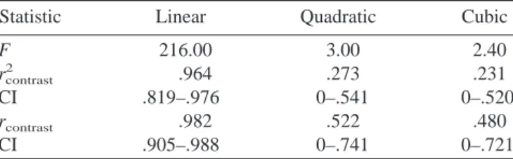
Table 3 shows the results of computing contrast correla-tions and the associated confidence intervals for linear, quadratic, and cubic trend. Some brief comments are in order. Note, first, that although the rcontrastvalues for
qua-dratic and cubic trends are appealingly high, the correspond-ing confidence intervals are quite wide and include zero. On the other hand, the confidence interval for the linear trend is very narrow.
The Relationship Between Confidence Intervals and Hypothesis Tests—Choosing the
Appropriate Interval
Confidence intervals on measures of effect size convey all the information in a hypothesis test, and more. If one selects an appropriate confidence interval, a hypothesis test may be performed simply by inspection. If the confidence interval excludes the null hypothesized value, then the null hypoth-esis is rejected.
In such applications, I recommend using the traditional two-sided confidence interval, rather than a one-sided interval (or confidence bound), regardless of whether the hypothesis test is one-sided or sided. When a two-sided confidence interval is used to perform the hypoth-esis test, the confidence level must be matched appropri-ately both to the type of hypothesis test and to the Type I error rate. Recall that the endpoints of the two-sided
confidence interval for a parameterat the 100(1⫺␣)%
confidence level are the values of that place the
ob-served statistic ˆ at the ␣/2 or 1 ⫺ ␣/2 cumulative
probability point. Suppose the upper and lower limits of
the 100(1 ⫺ ␣)% confidence interval are U and L,
re-spectively. Then ˆ is the rejection point at the ␣/2
sig-nificance level for one-sided hypothesis tests that is,
first, greater than or equal to U and, second, less than or equal to L. The observed statistic ˆis also equal to (a) the
upper rejection point for a two-sided test that⫽L at the
alpha level and (b) the lower rejection point for the
two-sided test that ⫽ U at the alpha level.
Conse-quently, the endpoints of the confidence interval
repre-sent two values of that the observed statistic would
barely reject in a two-sided test with significance level
alpha. These endpoints are also appropriate for testing
one-sided hypotheses at the␣/2 significance level.
The preceding paragraph implies a general rule of thumb: to use the confidence intervals to test a statistical hypothesis and to maintain a Type I error rate at alpha:
1. When testing a two-sided hypothesis at the alpha
level, use a 100(1⫺ ␣)% confidence interval.
2. When testing a one-sided hypothesis at the alpha
level, use a 100(1⫺ 2␣)% confidence interval.
Example 10: Consider a test of the hypothesis that⌿ ⫽
0, that is, that the RMSSE (as defined in Equation 12) in an ANOVA is zero. This hypothesis test is one-sided, because the RMSSE cannot be negative. To use a two-sided confidence interval to test this hypothesis at the
␣ ⫽ .05 significance level, one should examine the
100(1⫺ 2␣)%⫽ 90% confidence interval for ⌿. If the
confidence interval excludes zero, the null hypothesis will be rejected. This hypothesis test is equivalent to the standard ANOVA F test.
Example 11: Consider the test that the standardized effect
size Esin Equation 45 is precisely zero. This hypothesis test
is two-sided, because Escan be either positive or negative.
Consequently, to use a confidence interval to test this
hy-pothesis at the .05 level, a 100(1⫺␣)%⫽95% two-sided
confidence interval should be used, and the null hypothesis rejected only if both ends of the confidence interval are above zero or if both are below zero.
Example 12: Consider a situation in which one wishes
to establish that the standardized effect size Es in
Equa-tion 45 is small, and that smallness is defined as an absolute value less than 0.20. To establish smallness, one
must reject a hypothesis that Es is not small. Because Es
can be either positive or negative, Es can be not small in
two directions. The hypothesis that Es is not small can
therefore be tested with two simultaneous one-sided hy-pothesis tests,
H01: Esⱕ⫺0.20 versus Ha1: Es⬎⫺0.20 (52)
and
H02: Esⱖ0.20 versus Ha2: Es⬍0.20. (53)
These two hypotheses can both be tested simultaneously at the .05 level by constructing a 90% confidence interval and observing whether the lower end of the interval is above
⫺0.20 (to test the first one-sided hypothesis) and the upper
end of the interval is below 0.20. What this amounts to is
observing whether the entire interval is between⫺0.20 and
0.20. If so, the hypothesis that Esis not small is rejected, and smallness is indicated.
Table 3
Confidence Intervals (CIs) for Contrast Correlations
Statistic Linear Quadratic Cubic
F 216.00 3.00 2.40
rcontrast 2
.964 .273 .231
CI .819–.976 0–.541 0–.520
rcontrast .982 .522 .480 CI .905–.988 0–.741 0–.721
Tests of Minimal Effect Rationale and Method
In many situations, the null hypothesis of zero effect is inappropriate or can be misleading. For example, in R-S testing with extremely large sample sizes, a null hypoth-esis may be rejected consistently, with a very low prob-ability level, even when the population effect is small. Conversely, in A-S testing, the nil hypothesis of zero effect is often unreasonable, and the hypothesis the ex-perimenter probably wants to test is that the effect is trivial.
Tests of minimal effect are a partial solution to the problems caused by inappropriate testing of a nil hypoth-esis when the goal is to show that an effect is small. For example, if some “minimal reasonable” effect size can be specified, rejection of the hypothesis that the effect is less than or equal to this value is of practical importance whether or not the sample size is very large. In the traditional A-S situation, in which the experimenter is trying to show that an effect is trivial, the hypothesis that the effect is greater than or equal to a minimal reasonable value can be tested. Serlin and Lapsley (1993) discussed this latter notion in detail and gave numerical examples. In such cases, large sample size will work for, rather than against, the experimenter, because if the effect size is truly below a level that is of practical import, larger samples will yield greater power to demonstrate that fact by rejecting the null hypothesis that the effect is at or above a point of triviality.
The confidence intervals described in the preceding sec-tion can be used to test hypotheses of minimal effect: One simply observes whether the appropriately constructed con-fidence interval contains the target minimal reasonable value. For example, suppose you decide that an RMSSE of 0.25 constitutes a minimal reasonable effect. In other words, effects below that level may be ignored. Effects that are definitely above that level are nontrivial. If you wish to demonstrate that effects are trivial, you might test the hypotheses
H0:⌿ⱖ0.25; H1:⌿⬍0.25. (54)
On the other hand, if you wish to demonstrate that effects are definitely not trivial, you might test the hypotheses
H0:⌿ⱕ0.25; H1:⌿⬎0.25. (55)
In each case, rejecting the null hypothesis will support the goal in performing the test, and the problems inherent in A-S testing can be avoided.
A simple approach to simultaneously testing the two
hypotheses discussed above is to examine the 1 ⫺ 2␣
confidence interval for⌿ and see if it excludes 0.25. If
the entire confidence interval is above the point of triv-iality (i.e., 0.25), then the effect may be judged non-trivial. If the entire confidence interval is below the point of triviality, then the effect has been shown to be trivial. There is a strong similarity between using the effect size confidence interval in this way and the long tradition of bioequivalence testing.
Example 13: Suppose you have p⫽6 groups and n⫽75
per group. You observe an F statistic of F(5, 444)⫽2.28,
with p ⫽ .046, so the nil hypothesis of zero effects is
rejected at the .05 significance level. However, on
substan-tive grounds, you have decided that a value of⌿less than
0.25 can be ignored. To demonstrate triviality, you would attempt to reject the null hypothesis that⌿is greater than or equal to 0.25.
There are two approaches to performing the test. The first approach requires only a single calculation from the noncentral F distribution. Consider the cutoff value of 0.25. Using the result of Equation 12, one may convert
this to a value forvia the formula ⫽ (p⫺ 1)n⌿2⫽
(6⫺1)(75)(.252)⫽23.4375. The observed F statistic of
2.28 has a one-sided probability value of .0256 in the
noncentral F distribution with ⫽ 23.4375, and 5 and
444 degrees of freedom, so the null hypothesis is rejected at the .05 level, and the overall effects are declared trivial.
An alternative approach uses the confidence interval. Note that, because the test is one-sided, we use the 90%
confidence interval. The endpoints of the interval for
are 0.1028 and 20.3804. Using the result of Equation 12, we convert this confidence interval into a confidence interval for⌿by dividing the above endpoints by (p⫺1)n⫽375, then taking the square root. The resulting endpoints for the
confidence interval for ⌿ are 0.0166 and 0.2331. This
confidence interval excludes 0.25, so we can reject the
hypothesis that effects are nontrivial, that is,⌿ ⱖ 0.25, at
the .05 significance level. The advantage of using the con-fidence interval is that it provides us with an approximate indication of the precision of the estimation process while still allowing us to perform the hypothesis test.
Significant technical and theoretical issues surround the use of confidence intervals in this manner.
1. The choice of a numerical “point of triviality” for
a measure of omnibus effect size should not be treated as a mechanical selection from a small menu of “approved” choices. Rather, it should be considered carefully on the basis of the specific experimental design and the substantive aspects of the variables being measured and manipulated. Whereas .25 might be considered trivial in one experiment, it might be considered very important in another.
2. The power of both hypothesis tests must be ana-lyzed a priori to assess whether sample size is adequate. With low precision (i.e., a wide confi-dence interval), one might still have high power to demonstrate nontrivial effects if effects are large. However, it is virtually impossible to demonstrate triviality if precision is low, because the triviality point will be close to zero, and a wide confidence interval will not fit between zero and the triviality point.
Full consideration of the technical aspects of estimating the point of triviality, and precision of a parameter estimate and the resulting confidence interval, is beyond the scope (and length restrictions) of this article. However, in the next section, I discuss several theoretical issues that the sophis-ticated user should keep in mind.
Conclusions and Discussion
This article demonstrates that the F statistic in ANOVA contains information about standardized effect size, and its precision of estimation, that has not been made available in typical social science reports and is not reported by tradi-tional software packages. Yet this information can readily be calculated, using a few basic techniques.
The fact is, simply reporting an F statistic, and a proba-bility level attached to a hypothesis of nil effect, is so suboptimal that its continuance can no longer be justified, at least in a social science tradition that prides itself on em-piricism. A number of the field’s most influential commen-tators on social statistics have emphasized this and urged that, as researchers, we revise our approach to reporting the results of significance tests (e.g., see articles in Harlow, Mulaik, & Steiger, 1997).
Null hypothesis testing is the source of much contro-versy. I have tried to promote an eclectic, integrated point of view that resists the temptation to downgrade either the hypothesis testing or the interval estimation ap-proaches and emphasizes how they complement each other. Reviewers and other readers of the article have provided much food for thought and have raised several substantive criticisms that enriched my point of view considerably. In the following sections, I discuss some of the limitations of the procedures in this article, deal explicitly with several of the more common objections to my major suggestions, and then summarize my point of view and present some conclusions.
Statistical Limitations and Extensions of the Present Procedures
The procedures discussed in this article provide exact distributional results under standard ANOVA
assump-tions (independence, normality, and equal variances) and are easily calculated with modern software. However, they are restricted to (a) completely between-subjects fixed-effect ANOVA with (b) equal n per cell. The present article does not present procedures for dealing with the complications that result from unbalanced de-signs and/or repeated measures, nor does it discuss ex-tensions to random effects or mixed ANOVA models or to multivariate analyses.
In some cases, procedures for these other situations are already available. Consider, for example, the case of one-way random effects ANOVA. The treatment effects are
random variables with a variance of A
2
, and ⌿ may be
redefined asA/. A 100(1⫺ ␣)% confidence interval for
⌿may therefore be obtained in the equal n case by taking
the square root of the well-known (Glass & Hopkins, 1996,
p. 542) confidence interval forA
2
/2. One obtains, with p groups,
⌿lower⫽
冑
max冋
n⫺ 1冉
FobsF*␣/ 2⫺1
冊
, 0册
,⌿upper ⫽冑
max冋
n⫺1冉
FobsF*1⫺␣/ 2⫺
1
冊
, 0册
. (56)Fobsis the observed value of the F statistic, and F* is the
percentage point from the F distribution with p⫺ 1 and
p(n⫺1) degrees of freedom.
This approach can be generalized to more complicated designs. Burdick and Graybill (1992) discussed general
methods for obtaining exact confidence intervals for⌿and
related quantities in random effects models, both in the equal n and unbalanced cases. Computational procedures for the unbalanced case are much more complicated than for the case of equal n.
However, on close inspection, some extensions yield challenging complications that require careful analysis. Some examples are as follows.
1. In the unbalanced, fixed-effects case, the noncentrality
parameter is defined as follows:
⫽
冘
j⫽1
p
nj
冉
␣j
冊
2. (57)
Note that withdefined as in Equation 9, the quantity f2as
defined in Equation 10 represents the ratio of between-groups to within-group variance in a population with prob-ability of membership in the treatment groups proportional to the sample sizes in the ANOVA. There are situations in which this quantity is of interest (such as when the sampling plan reflects the relative size of natural subpopulations) and others in which it might not be. Cohen (1988, pp. 359 –361) discussed this point in detail.