Design of Structural Stand for High-Precision Optics Microscopy

MICROSCOPY

A Thesis presented to

the Faculty of California Polytechnic State University, San Luis Obispo

In Partial Fulfillment

of the Requirements for the Degree Master of Science in Mechanical Engineering

by

This work was performed under the auspices of the U.S. Department of Energy by Lawrence Livermore National Laboratory under Contract DE-AC52-07NA27344.

LLNL-TH-810933

COMMITTEE MEMBERSHIP

TITLE: Design of Structural Stand for High-Precision Optics Microscopy

AUTHOR: Sara Theresa Novell

DATE SUBMITTED: June 2020

COMMITTEE CHAIR: Kim Shollenberger, Ph.D.

Professor of Mechanical Engineering

Graduate Coordinator of Mechanical Engineering

COMMITTEE MEMBER: Charles Birdsong, Ph.D.

Professor of Mechanical Engineering

COMMITTEE MEMBER: Robert Plummer, M.S.

ABSTRACT

Design of Structural Stand for High-Precision Optics Microscopy Sara Theresa Novell

Lawrence Livermore National Lab (LLNL) is home to the National Ignition Facility (NIF), the world’s largest and most energetic laser. Each of the 192 beamlines contains dozens of large optics, which require offline damage inspection using large, raster-scanning microscopes. The primary microscope used to measure and characterize the optical damage sites has a precision level of 1 µm. Mounted in a class 100 clean room with a raised tile floor, the microscope is supported by a steel stand that structurally connects the microscope to the concrete ground. Due to ambient vibrations experienced in the system, the microscope is only able to reliably reach a 10-µm level of precision.

ACKNOWLEDGMENTS

This thesis was made possible by Lawrence Livermore National Laboratory, and I am thankful for the support from various engineers, technicians, administrators, and many others. I would specifically like to thank the following people for their various contributions throughout this project and my academic journey:

Robert Plummer, for creating this project, guiding me through it, and imparting invaluable engineering, writing, leadership, and problem-solving skills that I will carry with me for the rest of my life. Thank you for making this possible for me; your intelligence, patience, kindness, and support are attributes I will always strive to display.

Dain Holdener, for being kind, patient, and incredibly helpful in helping me navigate this project, collect data, and so much more. Thank you for taking time out of your busy workdays to answer my questions, provide technical and administrative support, and guide me both in this project and in my life.

Andy Jessop, Paul Geraghty, Stephen Hayes, and Paul Rosso for their strong technical guidance when collecting and analyzing data, borrowing and applying their equipment, and modeling designs in FEA.

TABLE OF CONTENTS

Page

LIST OF TABLES ... x

LIST OF FIGURES ... xi

NOMENCLATURE ... xvi

CHAPTER 1. INTRODUCTION ... 1

1.1 NIF Background ... 1

1.2 Optics Background ... 1

1.2.1 Optical Damage ... 2

1.2.2 The Optics Recycle Loop ... 6

1.3 The Need for Optical Microscopy ... 9

1.3.1 VIEW Microscope Specifications... 10

1.4 Cause of VIEW Limitations ... 11

1.4.1 Additional Considerations for Performance Improvements to the VIEW ... 14

1.5 Purpose of Study... 16

2. BACKGROUND ... 17

2.1 Vibrational Analysis ... 17

2.2 PSD Analysis ... 17

2.2.1 PSDs in MATLAB ... 18

2.2.2 Fourier Transforms ... 19

2.3.2 Window Type ... 30

2.3.3 PSD Strengths... 32

2.4 Vibrational Analysis and Modeling ... 32

2.4.1 Software Applications ... 32

2.5 Modal Analysis ... 33

2.6 Summary ... 35

3. DEVELOPING VIBRATIONAL REQUIREMENTS ... 36

3.1 Nikon Microscope Vibrational Requirements ... 36

3.1.1 Spectral Requirement Interpretation ... 37

3.1.2 Unregulated Bin Size Interpretation ... 39

3.2 Environmental Vibrational Criteria ... 41

3.3 Applying the Vibrational Criteria ... 45

3.4 OPF Analysis Setup ... 46

3.4.1 OPF Quiet Results Comparison ... 48

3.4.2 FEA Model Verification ... 53

3.4.3 Time Trial Results ... 57

3.5 OPF Results Summary ... 60

4. EXPERIMENTAL SETUP AND TESTING ... 61

4.1 Testing Equipment and Plan ... 62

4.1.1 Accelerometer Information ... 63

4.1.2 DAQ Information ... 65

4.1.3 Sampling Frequencies and Limitations ... 67

5. EXPERIMENTAL RESULTS AND ANALYSIS ... 72

5.1 Analysis Process ... 72

5.1.1 Processing Ambient/Quiet Data ... 74

5.1.2 Processing Shock Data ... 74

5.2 OAB Data Results ... 80

5.2.1 Data Validation ... 80

5.2.2 Wilcoxon Accelerometer Data ... 82

5.2.3 PCB Accelerometer Data ... 89

5.3 OAB Data Conclusions ... 93

6. MICROSCOPE STAND DESIGN ... 95

6.1 Model Validation ... 96

6.2 Compliant/Flexible Designs ... 100

6.2.1 2x2” Basic Structure ... 100

6.2.2 2x2” Diagonal Structure ... 107

6.3 Stiff Designs ... 115

6.3.1 6x6” Basic Structure ... 116

6.3.2 6x6” Diagonal Structure ... 120

7. CONCLUSION ... 129

7.1 Thesis Goals and Approach ... 129

7.2 Analytical Results ... 130

7.3 Recommendations ... 131

APPENDICES

A. PSD TO VC REQUIREMENTS: MATLAB FUNCTION ... 137

B. OPF STAND HAND CALCULATIONS ... 139

C. EXPERIMENTAL EQUIPMENT MANUALS ... 142

C.1 Selection from National Instruments (NI) DAQ (NI 9234) Datasheet... 142

C.2 Selection from NI DAQ Chassis (NI cDAQ 9178) Datasheet ... 146

C.3 Selection from Wilcoxon Accelerometer (731A) Datasheet ... 148

C.4 Selection from PCB Accelerometer (356B18) Datasheet ... 151

D. CLEAN ROOM BUILDING DRAWINGS ... 152

D.1 OAB Building Drawing: PLZ-97-681-E, Sheet No. S2-1 ... 152

D.2 OPF Building Drawing: PLZ74-391-093JA, Sheet No. S-32 ... 154

E. MATLAB CODE TO PROCESS ACCELEROMETER DATA ... 155

F. SIMPLE BEAM HAND CALCULATIONS ... 161

LIST OF TABLES

Page

Table 2-1. Octave and one-third octave bands [19, 20] ... 26

Table 3-1. Vibrational requirements set by Nikon ... 36

Table 3-2. Descriptions of criterion curves [31] ... 41

Table 3-3. Modal frequencies of the OPF stand ... 49

Table 3-4. Description of each modal frequency of OPF stand ... 55

Table 6-1. Modal analysis results of basic beam ... 97

Table 6-2. Modal analysis results of 2x2” box tube structure ... 102

Table 6-3. Modal analysis results of 2x2” box tube structure with diagonal supports ... 108

Table 6-4. Modal analysis results of 6x6” box tube structure ... 117

LIST OF FIGURES

Page

Figure 1-1. Optical damage site from an optic on NIF [3] ... 2

Figure 1-2. Damage initiation site on a fused silica optical surface showing how the fused silica melts when exposed to high fluence [3] ... 3

Figure 1-3. Image of filamentation tracks inside the bulk of an optic [3] ... 4

Figure 1-4. Laser light diffracted through a diffraction grating, with a higher k-value indicating a lower percent energy of the original lower beam [4]... 5

Figure 1-5. An outline of the optics recycle loop [5]... 6

Figure 1-6. Photo of FODI inside the NIF target chamber [5] ... 7

Figure 1-7. Mitigated damage site [9] ... 9

Figure 1-8. Micrographs of a damage site before and after CO2 laser mitigation [7] ... 9

Figure 1-9. Summit drawing of the VIEW, with dimensions given in millimeters [8] ... 11

Figure 1-10. VIEW microscope in clean room ... 12

Figure 1-11. The underfloor plenum of a class 100 clean room at LLNL... 13

Figure 1-12. Simplified CAD of stand on which the VIEW microscope is mounted in the OPF ... 14

Figure 1-13. LLNL maps showing the relative locations of the OAB and the OPF to the NIF building ... 15

Figure 2-1. Identical vibrational data processed with (a) DFT and (b) PSD ... 21

Figure 2-2. Graphical display of Welch’s method [13] ... 23

Figure 2-4. Graph showing lowest one-third octave band frequencies based on PSD bin

size ... 28

Figure 2-5. PSD calculation with (a) 0% and 50% overlap, (b) 50% and 75% overlap ... 30

Figure 3-1. Data processed to compare to spectral requirements interpretation ... 38

Figure 3-2. Graphs showing same frequency data, with (a) 5 Hz bins, and (b) 500 Hz bins ... 40

Figure 3-3. VC curves in (a) US Customary [30] and (b) SI units [29] ... 44

Figure 3-4. How MATLAB and ANSYS Mechanical analyze the OPF stand... 46

Figure 3-5. OPF stand on ANSYS Mechanical with axes shown... 47

Figure 3-6. Mesh created in ANSYS mechanical ... 48

Figure 3-7. Transmissibility curves for various damping ratios [31] ... 50

Figure 3-8. OPF stand vibrational data in (a) x-direction, (b) y-direction, and (c) z-direction ... 52

Figure 3-9. View of the (a) original mesh and (b) refined mesh ... 54

Figure 3-10. OPF stand with refined mesh vibrational results in (a) x-direction, (b) y-direction, and (c) z-direction ... 57

Figure 3-11. VC results from each time trial in (a) x-, (b) y-, and (c) z-direction ... 59

Figure 4-1. OPF testing and analysis flowchart ... 61

Figure 4-2. OAB testing and analysis flowchart ... 62

Figure 4-3. Three Wilcoxon accelerometers on triaxial mounting block ... 64

Figure 4-4. NI DAQ during testing setup ... 66

Figure 4-5. Aliasing, shown in this graph, results in inaccurate data interpretation [35] ... 67

Figure 5-1. Vibrational data taken as a function of time to show (a) ambient and (b) shock

cases ... 73

Figure 5-2. Shock and quiet data vibrational signatures from the OAB ... 75

Figure 5-3. PSD comparison of shock data and quiet data ... 76

Figure 5-4. Singular first peak from the shock data isolated and compared to quiet data ... 77

Figure 5-5. PSD results on small section of peak shock data ... 78

Figure 5-6. PSD result on shock peak when DFT length was increased ... 79

Figure 5-7. Data collected in the (a) GDS lab and (b) OAB lab ... 82

Figure 5-8. PSD results taken with the Wilcoxon accelerometer in the (from top to bottom) x-direction, y-direction, and z-direction ... 83

Figure 5-9. Wilcoxon VC results in (a) x-direction, (b) y-direction, and (c) z-direction ... 85

Figure 5-10. PSD results from Wilcoxon set to (a) 100 V/g and (b) 1000 V/g ... 86

Figure 5-11. Sensitivity analysis in (a) x-direction, (b) y-direction, and (c) z-direction ... 88

Figure 5-12. PSD of PCB accelerometer data ... 90

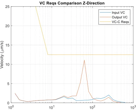
Figure 5-13. PCB accelerometer data converted to compare to VC-C requirements in the (a) x-direction, (b) y-direction, and (c) z-direction ... 92

Figure 6-1. Location of PSD inputs and output on microscope stand model ... 95

Figure 6-2. Project schematic from ANSYS showing all three applied modules... 96

Figure 6-3. Simple ANSYS model of a cantilever beam with a point mass on the top ... 96

Figure 6-4. Simple model input and output PSD in (a) x- direction, (b) y- direction, and (c) z-direction ... 99

Figure 6-5. Thick wall 2x2” box tubing design with the lowest stiffness ... 100

Figure 6-7. Transmissibility graph of 2x2” box tube stand normalized to first mode ... 104

Figure 6-8. VC results of 2x2” box tube stand in (a) x- axis, (b) y- axis, and (c) z-axis... 106

Figure 6-9. Thick wall 2x2” box tubing design with diagonal supports ... 107

Figure 6-10. 2x2” diagonally supported design with mesh shown ... 108

Figure 6-11. Transmissibility graph of 2x2” box tube diagonal stand ... 109

Figure 6-12. Transmissibility graph of 2x2” box tube diagonal stand with identical transverse PSD inputs... 111

Figure 6-13. Mesh for the 2x2” diagonally supported stand and exact PSD output point ... 112

Figure 6-14. VC results of 2x2” box tube stand with diagonal supports in (a) x-direction, (b) y-direction, and (c) z-direction ... 114

Figure 6-15. The cause of the y-direction output attenuation effect seen in the 2x2” diagonally supported design [39] ... 115

Figure 6-16. Thick wall 6x6” box tubing design ... 116

Figure 6-17. 6x6” model with mesh shown ... 117

Figure 6-18. Transmissibility graph of 6x6” box tube stand near first mode ... 118

Figure 6-19. VC results of 6x6” box tube stand in (a) x-axis, (b) y axis, and (c) z- axis ... 120

Figure 6-20. Thick wall 6x6” box tubing design with diagonal supports ... 121

Figure 6-21. Mesh for 6x6” diagonally supported model ... 121

Figure 6-22. Transmissibility graph of diagonally supported 6x6” box tube stand ... 123

Figure 6-23. Transmissibility graph of diagonally supported 6x6” box tube stand normalized to first modal frequency of 83 Hz ... 124

Figure 6-25. VC results of 6x6” box tube diagonally supported stand in (a) x-direction,

NOMENCLATURE

AR..……….…….……….………...………Antireflection CAD..……….……….………Computer Aided Design DAQ..……….………..………..Data Acquisition System DOF..……….………..………...Degree of Freedom DFT..……….………..………...Discrete Fourier Transform FEA..……….………..………Finite Element Analysis FFT..……….………....………Fast Fourier Transform FODI...………..………..Final Optics Damage Inspection GDS..……….………..………...Grating Debris Shield

1. INTRODUCTION 1.1 NIF Background

Located at Lawrence Livermore National Laboratory (LLNL), the National Ignition Facility (NIF) is the world’s largest and most energetic laser [1]. NIF is comprised of 192 beams that propagate through thousands of large, precision optics in order to converge on a single target at the correct power, energy, frequency, polarization, focus, and more. The purpose of the NIF is to provide a world-class research facility for conducting experiments related to inertial confinement fusion (ICF). With a goal of achieving thermonuclear burn from fusing hydrogen together, the mission of NIF focuses on High Energy Density (HED) physics, national security, basic science research, and clean energy. After every shot, operational data is used to optimize future performance of the laser and its diagnostics. The optics that comprise the laser form a critical piece of this performance optimization, and this learning and development keep NIF on the cutting edge of laser research in the world.

The optics within the NIF beamline are largely made of potassium dihydrogen phosphate (KDP) or fused silica. They are used not only to adjust beam properties but also to play a critical role in diverting some parts of the beams to diagnostics. These diagnostics, or measuring devices, are used to calculate the beam-to-beam power balance and determine laser performance. Therefore, the condition and development of the optics on the NIF are crucial to its success.

1.2 Optics Background

(OMST) group at the Laboratory. Optics on the NIF can vary greatly in size, weight, and shape because they each provide unique functions.

1.2.1 Optical Damage

Optics must be closely monitored and actively managed due to damage caused by NIF shots. NIF operates at 1.8 MJ and 500 TW and is converted from its front-end transport wavelength of 1053 nm (IR) to 351 nm (UV) just prior to being delivered to the target [1]. This power and fluence (energy per area) can lead to damage, especially in the UV section of the beam path. Damage sites are areas on the optic that have sustained damage and vary in size up to a few mm; visually, they appear as small pits or discontinuities on the optical surface, as shown in Figure 1-1.

Figure 1-1. Optical damage site from an optic on NIF [3]

There are several different optical damage mechanisms, and each one results from one of the three possible ways in which light can propagate: transmission, absorption, or reflection. As the NIF laser light travels through the optics, the damage is caused by the laser fluence, intensity (power per area), or debris. Debris on optic surfaces causes the most damage sites, and the sites can be three to four times larger than the debris itself [3]. The debris’ thermal conductivity can be higher than that of the optic’s material; thus, the debris absorbs more heat from the laser and induces cracking of the optical substrate. Debris is the leading contributor of optical damage as the NIF begins to mature, and this mechanism remains a challenge to manage. Nonetheless, light absorption can also cause damage to optics even without debris due to other extrinsic absorbing precursors such as facture surfaces and nm level chemical impurities on or just below surface of the optic and foreign bulk inclusions. Figure 1-2 shows a damage site of melted fused silica.

Figure 1-2. Damage initiation site on a fused silica optical surface showing how the fused silica melts when exposed to high fluence [3]

optic that can enhance power of the laser into a specific spot within the bulk, or middle, of the optic [3]. Figure 1-3 shows an image of the large amount of damage caused by filamentation tracks on the bulk of an optic.

Figure 1-3. Image of filamentation tracks inside the bulk of an optic [3]

Figure 1-4. Laser light diffracted through a diffraction grating, with a higher k-value indicating a lower percent energy of the original lower beam [4]

placement and adjustable alignment), there are still unavoidable ghost locations that result in damage on the optics [3].

The effects of the damage sites must be mitigated, and when located and characterized, the damage sites are repaired in an offline facility using a novel laser ablation protocol. Knowing where the damage sites are and what they look like is necessary for success on the NIF.

1.2.2 The Optics Recycle Loop

In order to mitigate the effect of the damage sites, they first need to be located. This begins the recycling loop of optics, which is simplified and outlined in Figure 1-5, and according to the source of this figure, “blue rectangles indicate steps required for routine operation of the laser, blue diamonds are decision points related to damage, and yellow rectangles are steps associated with fabricating damage-resistant optics” [5].

To determine if an optic is damaged enough to be taken off NIF, a precision imaging system called Final Optics Damage Inspection (FODI), the in-situ optic inspection in the optics recycle loop seen in Figure 1-5, uses custom-developed machine learning algorithms and image analysis to determine which optics need to be checked and the location of each damage site [6]. It does this through a coordinated network of fiber optic light and a precision telescope [6]. FODI enables automation and shot cycle efficiencies of NIF (i.e. more shots per optic before they must be taken off of the beamline); veritably, FODI is in large part the reason why the laser can run at such a high energy. The development of FODI’s ability to assess the damage systematically and routinely on the final optics is an unparalleled technology that can reliably track damage sites down to the size of 10 µm [6]. Without FODI, it would present an immense operational challenge to determine, predict, and manage the optical damage accurately to enable NIF to continually operate at its peak fluence and power. A photo of FODI is shown in Figure 1-6.

Once FODI has determined that an optic needs to be removed due to damage, the optic is transported to the Optics Processing Facility (OPF) where it is inspected on large microscopes to verify that the FODI data is accurate, characterize the damage sites with higher resolution, and use this information to continually improve the accuracy of the FODI. In characterizing the damage sites, the microscopes determine the location sites, size, depth, and morphology. Then, the optic is sent to the Optic Mitigation Facility (OMF) where the damage sites are ablated and mitigated.

Figure 1-7. Mitigated damage site [9]

Figure 1-8. Micrographs of a damage site before and after CO2 laser mitigation [7] 1.3 The Need for Optical Microscopy

As mentioned previously, an imperative step in the recycle loop is the microscopy to characterize the damage sites. The OPF uses high-resolution, full aperture, raster-scanning microscopes that are programmed with LLNL-made scripts to map the entire optic surface to create a full resolution image.

measures about two times faster than the VIEW due to its ease of use and ability to implement external programming; in fact, the Nikon lacks the need to focus on every damage site in order to capture the correct image, saving significant operating time. However, its stage capacity is limited to 110 pounds. The VIEW can accommodate optics up to 220 pounds, which encapsulates nearly all NIF large optics, as well as measure to a single-micron scale like the Nikon. However, it is unable to reliably reach that level of resolution in practice because of ambient vibrations in the room in which it is fielded. Maintaining the capability to characterize the heaviest optics while increasing operational throughput is an important goal to OMST.

1.3.1 VIEW Microscope Specifications

The VIEW microscope, shown in the vendor-provided drawing in Figure 1-9, is equipped with an optical stage made from glass and mounted on a large granite table, which contributes greatly to the 2200 lb. weight of the machine. Based on the original specifications from the vendor, the VIEW is only able to hold optics with weights of up to 110 pounds. In order to enable the microscopy of the largest and heaviest NIF optics, testing was performed by LLNL in conjunction with the vendor to qualify the stage for an increased capacity of 220 pounds. Now, the stage capacity has been increased to allow 220-pound optics; however, Summit did not make guarantees about lifetime or precision after this qualification.

Figure 1-9. Summit drawing of the VIEW, with dimensions given in millimeters [8] 1.4 Cause of VIEW Limitations

Figure 1-10. VIEW microscope in clean room

Figure 1-11. The underfloor plenum of a class 100 clean room at LLNL

Figure 1-12. Simplified CAD of stand on which the VIEW microscope is mounted in the OPF

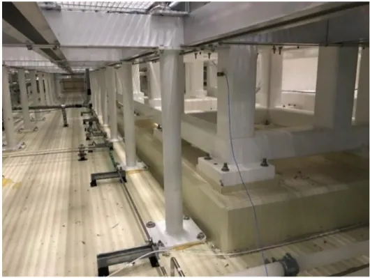
A further study into the design of the current VIEW stand in the OPF highlights its simplicity. Although effective for the imaging of larger damage sites, the stand does not include any cross supports which could increase stiffness in the x- or y-directions as well as help prevent rotation in all axes. Furthermore, vibrational studies done in the clean rooms can indicate if a stand needs to account for stiffness or damping, and these decisions can be based on well-established vibrational criteria. It is apparent that a more sophisticated design could be engineered that would allow for the VIEW microscope to yield higher resolution images and results, thus aligning the microscope’s abilities with OMST’s goals. 1.4.1 Additional Considerations for Performance Improvements to the VIEW

realize the operational efficiencies and resource savings of improving the lifetime of the optics. Formerly, damage sites on the order of 50 microns were mitigated, but there is now a concerted effort to mitigate damage sites as small as 10 microns. As a result, microscopes that measure and characterize the damage sites are becoming more impacted.

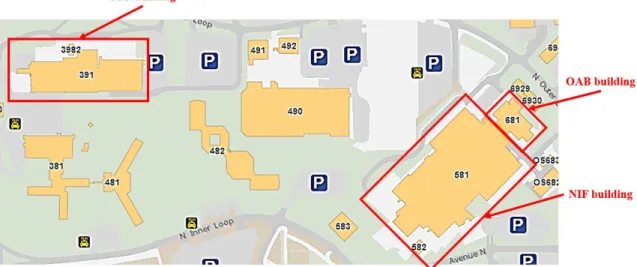
With the increased demand on these microscopes comes the increased amount of physical optic transportation. Currently, the VIEW microscope resides in the OPF, which is located several buildings away from the NIF. The new stand is being proposed to be mounted in the OAB, which is connected to the NIF building, so the VIEW microscope can be located much closer to the optics, thus limiting the distance the optics need to move. The more an optic is moved around, the more likely it is to get inadvertently damaged due to transport and handling—as opposed to performance online—so optimizing the location of optic metrology is an ancillary benefit of adding a VIEW microscope closer to the NIF building. A map of these buildings to show their relative locations can be seen in Figure 1-13.

The VIEW microscope can support and measure heavier optics from the NIF. At the beginning of the beam line, the laser is in the infrared (IR) spectrum and propagated multiple times through large optics known as amplifier slabs, which provide 99.9% of the NIF’s energy [1]. Since this is the low-power part of the beamline, the slabs’ optical coatings are not nearly as affected. As a result, the coatings and substrates sustain significantly less damage than the optics at the UV spectrum of the beamline. Even so, there is a desire to perform metrology on these amplifier slabs to characterize the surface. Given that NIF has been in operation for over ten years, there are studies being undertaken internally to understand the effects of laser operations on the amplifier slabs. A critical part of understanding amplifier performance is to characterize the surface using high-resolution, full aperture microscopes like the VIEW, which has the requisite stage capacity to measure the slabs. The demand on this microscope is ever increasing, and OMST must provide this capability.

1.5 Purpose of Study

2. BACKGROUND 2.1. Vibrational Analysis

Vibrational analysis is a fundamental subject in the study of mechanical engineering, and there are various paths of study possible based on measured inputs and desired outputs. In this project, the vibrational analysis selected is a Power Spectral Density (PSD) because of its abilities to dissect random vibrations and present results and vibrational trends in meaningful ways. By engineering definition, the vibrations measured are categorized as random vibrations. To clarify, this means that the measurements of a system taken at one point in time are statistically similar to measurements of the same system taken in the future [10], as opposed to stationary vibrations, which are able to be found using a “function, mapping or some other recipe or algorithm” [11]. PSD mathematics are rooted in developments and manipulation of Fourier transforms and statistics and can be analyzed in programming languages such as MATLAB, which is employed in this project.

2.2. PSD Analysis

2.2.1 PSDs in MATLAB

In MATLAB, Welch’s method is a common PSD analysis tool, and the mathematical specifics of Welch’s method will be discussed in section 2.3. Looking at the inputs and outputs of a PSD in a programming language provides an introductory overview of what each variable signifies in the calculation.

The built-in pwelch function in MATLAB calculates the PSD using Welch’s method, and is shown in Equation 2-1 below, where variables in bracket are outputs, and the variables in parenthesis are inputs.

[𝑝𝑥𝑥, 𝑓] = 𝑝𝑤𝑒𝑙𝑐ℎ(𝑥, 𝑤𝑖𝑛𝑑𝑜𝑤, 𝑛𝑜𝑣𝑒𝑟𝑙𝑎𝑝, 𝑓, 𝑓𝑠) (2-1)

pxx is the PSD output vector, f is the output frequency vector, x is the time-based input

vibrational amplitude vector (typically acceleration, but can be velocity or displacement), window is the window type, noverlap is the percent overlap in each frequency bin, f input

is the value of Discrete Fourier Transform (DFT) length, and fs is the value of the sampling

frequency at which x was collected [13]. The size of each output vector is the same, but this length depends on the percent overlap and sampling frequency, as shown in Equation 2-2. All the data in x is calculated and averaged into a PSD to fit into this length.

𝑙𝑒𝑛𝑔𝑡ℎ(𝑝_𝑥𝑥) = (% 𝑜𝑣𝑒𝑟𝑙𝑎𝑝) ∗ 𝑓𝑠 (2-2)

2.2.2 Fourier Transforms

Put simply, a PSD converts amplitude data per time into a mean-squared-value of acceleration per frequency. This calculation begins with a Fourier transform of the time-domain data to make it spectral data (i.e. a function of frequency) [13]. A Fourier transform is a mathematical calculation that implements the Fourier series assumption that any function or signal can be broken up into a summation of sine and cosine (periodic) functions. By expanding this foundation and integrating the Fourier series of infinite length, the Fourier transform is created. A Fourier transform can be thought of as the discrete analog of a Fourier series, and, when executed, outputs a function or signal into its individual frequencies [14]. Equation 2-3 shows how a Fourier transform takes a time-based function f(t) and turns it into a complex function of frequency (w) using an infinite integral, where i is the imaginary variable.

𝐹(𝑤) = ∫ 𝑓(𝑡)𝑒−𝑖𝑤𝑡 ∞

−∞

𝑑𝑡 (2-3)

For a finite (i.e. collected) data series, a discrete Fourier transform (DFT) must be implemented. The key difference between a DFT and the full Fourier transform is the infinite integral from the Fourier transform is replaced with a summation along the length of the data collected. In this case, Equation 2-4 below is used on data x (which is a function of time, t of index n) of length N and index k (where k = 0, 1, 2,…, N-1) to make a function of frequency w [15].

𝐹(𝑤_𝑘) = ∑ 𝑥(𝑡_𝑛)𝑒−𝑖𝑤𝑘𝑡𝑛

𝑁−1

𝑛=0

Because the PSD calculations are done in MATLAB (i.e. in a programming language), a Fast Fourier Transform (FFT)—which is an algorithm to quickly and efficient find a DFT—calculates the DFT.

For some vibrational studies, the DFT calculations are all that is necessary to ascertain accurate results, as certain simple vibration types—such as those with a singular, periodic vibrational source—can be understood well after this transform; however, the vibrations measured in this project are random in nature and must be processed further.

(a)

(b)

2.3 Calculation and considerations of the PSD

Once the DFT is complete and the data is in the frequency domain, the Fourier transform result is squared and averaged over a certain frequency band, or bin size; finally, it is presented and truncated using a statistically developed windowing function. Squaring the data allows the magnitudes to be compared since the vibrations are measured directionally both positive and negative; also, squaring converts both the vibration into power and the complex data into a real data structure. Averaging the data normalizes the magnitude and eliminates off-normal events from the measured data that can cause erroneous peaks in the results. Deciding the window type gives control over how the result is presented and is critical for making valid conclusions. In formulaic form (shown in Equation 2-5), Welch’s method outputs a PSD, g, as a function of frequency f, where Δt is the time step between collected data points, M is the number of segments—or ensembles— selected from the time data, ξ is the modulus (i.e. distance from zero) of the segments [13]. Like the DFT calculation in Equation 2-4, k is an indexing variable for the DFT starting at zero and ending at n, and m is the indexing variable for the PSD averaging starting at one.

𝑔̂(𝑓_𝑘) =2∆𝑡

𝑀𝑛 ∑ |𝜉𝑘𝑚|

2 𝑀

𝑚=1

(2-5)

Looking back at Equation 2-1, there are some similarities of the inputs. In that MATLAB equation, fs is 1/Δt in this equation, f input is the DFT length n, and x is the

time-based data on which the DFT is done to result in ξ.

x(t) are changed into a magnitude function of frequency (ξkm), and eventually a full PSD,

gxx(fk). The ensembles are either chosen based on what needs to be analyzed or are selected

at random in order to gather enough data to create a PSD.

Figure 2-2. Graphical display of Welch’s method [13]

Figure 2-3. PSD found using (clockwise from top left) Periodogram method, Welch method, Blackman-Turkey (B-T) method, and multi-taper method [16]

Along with the calculation itself, there are other decisions, namely bin size and percent overlap, that must be made in order to complete the PSD analysis in MATLAB. 2.3.1 Bin Size and Overlap

frequency resolution =𝑓𝑠

𝑁 (2-6)

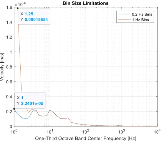
Although there is no absolute standard way to decide what a bin size should be— because each case is different—there are certain recommendations. It is always suggested that the DFT length is longer than the data collected in order to avoid unnecessarily truncating the data [17]. As a first pass, it is typical to have a DFT length be an integer power of two that is above the length of the data set; in practice, that means if the data length is 1000, for example, the DFT length should be selected as 1024, or 210 [17]. However, when taken in consideration of the frequency resolution in Equation 2-6, this “power of two” rule cannot hold up in a couple different scenarios. First, if low output frequencies are desired, a higher precision frequency resolution is necessary, and the Fourier transform length must be longer. This concept will be discussed further later in this section. Second, if many data points are collected, the power-of-two may be too high and can overload the coding program. For example, if 4.8 million data points are collected, the next largest power of two is 223 _{(over 8.3 million), which is much higher than necessary} and will slow down or likely crash the program. The decision of DFT length depends on each application and can vary based on desired outputs.

One-third octaves are derived by breaking each octave into One-thirds, as shown in Table 2-1 [19]. For many applications, the band number—or index—begins at 15 (i.e. 31.5 Hz) rather than 0 (i.e. 1 Hz); however, this application requires all the ANSI standard one-third octave center frequencies, so this table is extrapolated to display those lower frequencies. To find the one-third octave center frequency mathematically, Equation 2-7 is used, where n is the band number.

𝑓 = 2𝑛/3 (2-7)

Table 2-1. Octave and one-third octave bands [19, 20]

Band Number Octave Center Frequency (Hz)

One-third Octave Center Frequency (Hz) 31 30 29 1000 1200 1000 800 28 27 26 500 630 500 400 25 24 23 250 320 250 200 22 21 20 125 160 125 100 19 18 17 63 80 63 50

15 14

31.5 31.5

25 13 12 11 16 20 16 12.5 10 9 8 8 10 8 6.3 7 6 5 4 5 4 3.15 4 3 2 2 2.5 2 1.6 1

0 1

1.25 1

Figure 2-4. Graph showing lowest one-third octave band frequencies based on PSD bin size

without benefit [17]. Figure 2-5 below shows how changing from 0% to 50% overlap attenuates data and normalizes out some peaks and valleys, but the difference between a 50% and 75% overlap is negligible.

(b)

Figure 2-5. PSD calculation with (a) 0% and 50% overlap and (b) 50% and 75% overlap 2.3.2 Window Type

The final specification that must be set to complete the PSD calculations is a window type. Selecting a window, otherwise known as windowing, truncates data and presents it in a clear manner. The necessity of window selection stems from the limited data sample collected during testing; if the data is not windowed properly, the results of the PSD can be drastically misleading [21]. In this definition, “limited data” is any finite amount of data collected, and this classification indicates that complete vibrational trends may not have been fully tracked during the allotted testing time [22].

expected to start and end at zero as well as have an integer number of cycles, and this is nearly impossible to collect in real, experimental data [23]. To reduce the number of discontinuities resulting from the data being cutoff mid-cycle (i.e. mid-sinusoid) and starting at a different number, windowing “matches as many orders of the derivative as possible at the boundary.” [22]. Essentially, windowing matches the value, slope, and concavity of the windowed function to the collected data at its boundaries.

Spectral leakage is defined as artificially high frequency signals resulting from DFT calculations and seemingly missing time data [24]. It is a remnant of the DFT and how a finite sampling time and frequency cannot properly analyze signals that are not integer multiples of the frequency resolution. This means there is a void of time data to the DFT input, which is called leakage in the spectrum domain. The result of spectral leakage is frequency content that should be zero but is instead non-zero. Although increasing the sampling frequency can reduce this problem because it increases the chance of having integer multiples of the DFT, windowing is the only way to entirely remove this effect [24]. Windowing functions by multiplying the DFT result by a specific windowing function, making the signal go to zero at the correct frequencies by making the function appear more periodic.

to see trends—without attenuating peaks that remain statistically relevant [21]. Furthermore, the Hann window function and its derivative are continuous, and no additional data storage is necessary because it is drawn from the cosine data in the already-completed DFT—making the Hann window an efficient calculation [22].

2.3.3 PSD Strengths

As mentioned, PSD analysis can take the arbitrariness out of random vibrational data and output meaningful trends, making it the optimal analysis option for this project. Prior research substantiates the belief that a PSD is the top analysis option when “random effects obscure the underlying phenomenon” [21]. The laboratories in which the VIEW microscope is placed (i.e. the OPF and OAB) have random vibrations due to HVAC, equipment, and operators. These random vibrations create noise and hide the true trends in the building, and a DFT alone is not enough to clarify and scrutinize the data. A PSD takes the vibrational data from the microscopy environments of interest and turns it into clear and purposeful trends that guide further testing, designs, and analysis.

2.4 Vibrational Analysis and Modeling 2.4.1 Software Applications

ANSYS has various software modules for vibrational analysis, and in this project, the “Random Vibration” module was utilized. As with most vibrational modules, the “Random Vibration” module stems from modal analysis, which calculates the modes and mode shapes of the structure being analyzed.

2.5 Modal Analysis

Modal analysis is a fundamental strategy implemented to complete vibrational analysis and find dynamic properties of a structure in the frequency domain [25]. Often, modal frequencies are referred to as natural frequencies or resonant frequencies of a system because the object will resonate, or have amplified displacements, at these frequencies. The fundamental relationship for deriving natural frequency of a single degree of freedom (SDOF) system undergoing simple harmonic motion (SHM) is shown in Equation 2-8, where k is the spring constant and m is the mass of the object of interest.

𝑤𝑛 = √

𝑘 𝑚

(2-8)

[𝑀][Ü] + [𝐶][𝑈̇] + [𝐾][𝑈] = [𝐹] (2-9)

This equation is the general EOM for vibrational motion, and it is simplified for modal analysis by assuming damping is negligible because natural frequencies are a function of mass and stiffness. Also, forced responses are not necessary for modal analysis, so the force vector goes to zero. The result of these simplifications can be seen in Equation 2-10.

[𝑀][Ü] + [𝐾][𝑈] = 0 (2-10)

To find the modal frequencies, harmonic motion is assumed [26], which means the acceleration vector can be written as displacement multiplied by the eigenvalue of the new [M] and [K] matrix, simplified and shown in Equation 2-11. From this formula, λ can be calculated, where λ is the square of the modal frequencies.

[𝑀𝜆 + 𝐾][𝑈] = 0 (2-11)

Based on this formula, there is a modal frequency for each DOF; therefore, there are infinitely many modes for a real system.

Once the eigenvalues are calculated, the mode shapes can be found. Mode shapes describe how a system physically moves at a certain mode by calculating the relative displacement of each mass degree of freedom for a given frequency. They can be found using Equation 2-12 below, where ϕ is the eigenvector (i.e. mode shape) for the specific eigenvalue or given modal frequency.

This eigenvector can then be plotted as normalized displacements at each mass, which results in the mode shape caused by the input modal frequency, λ [26]. When done on a computer in FEA software, these modes and mode shapes can be found quickly and provide the basis for further vibrational analysis.

2.6 Summary

3. DEVELOPLING VIBRATIONAL REQUIREMENTS

The VIEW microscope is not meeting its intended precision measurement specifications due to ambient vibrations, and Summit does not provide any vibrational requirements for the environment in which the microscope is to be fielded. Nikon (the manufacturer of the other microscope that measures NIF optics) does specify vibrational requirements, but they are unexacting as they can be interpreted in different ways. Therefore, explicit vibrational requirements must be outlined before a new microscope stand can be designed, as those requirements will define what specifications the stand must meet.

3.1 Nikon Microscope Vibrational Requirements

Nikon outlines the vibrational specifications seen in Table 3-1, and at first glance they can seem straightforward; however, there are several different ways these specifications can be interpreted. The possibilities that will be discussed further in this thesis include analysis as a spectral requirement or analysis as averages with any undefined variation of bin size.

Table 3-1. Vibrational requirements set by Nikon

Frequency Range Requirement

10 Hz and lower Amplitude: 3 µmp-p or lower

10 Hz to 1000 Hz Acceleration: 0.012 m/s2 or lower

the sample was taken for 19 seconds. An important note is that not all these interpretations are considered standard within the vibration community; the following discussion is rather intended to highlight the ambiguity of the Nikon requirements.

3.1.1 Spectral Requirement Interpretation

The most likely way to interpret these is as a spectral requirement, or a function of frequency. This would mean that acceleration data is collected and, using a DFT, calculated into a function of frequency. Then, by assuming simple harmonic motion, the acceleration can be converted into displacement (amplitude) and velocity. Equations 3-1a and 3-1b below outline how velocity (v) and displacement (d) can be calculated from acceleration (a), where f is frequency [27].

𝑣 = 𝑎 2𝜋𝑓

(3-1a)

𝑑 = 𝑣 𝜋𝑓

(3-1b)

(a)

(b)

These graphs show that in the low end of the frequency domain, the microscope would not meet the vibrational requirements; however, it is well below the requirements at 1 Hz or higher. This happens because lower frequencies result in higher displacements, as lower frequencies propagate further since “they do not lose as much energy though joints, cracks, or any other irregularities in a material.” [28]. This means that low frequency vibrations can be shaking a structure even from far away, whereas a high frequency source attenuates. As a result, the displacement magnitudes are much higher at low frequencies. 3.1.2 Unregulated Bin Size Interpretation

(a)

(b)

The vibrational requirements given by Nikon are not sufficiently clear and can skew the results; therefore, more rigorous and standardized requirements must be implemented. 3.2 Environmental Vibrational Criteria

One highly developed vibrational requirement methodology is the vibrational criterion (VC) curves. These curves are “commonly used in the design of facilities which house vibration-sensitive instruments and tools” because they are comprehensive and well-studied [29]. Each curve is labeled as VC-x—where x is any letter A to E—and each curve describes a certain velocity vibration criterion, described below in Table 3-2. These velocities refer to vibrations as an input to the base, or floor, on which equipment is placed; in this project, this would mean the top of the microscope stand. This table also includes some International Standards Organization (ISO) standards, which are also velocity-based, for reference to real-world vibrations in terms of how they would generally be perceived by people.

Table 3-2. Descriptions of criterion curves [31] Criterion Curve Max Level (micro-in/sec) Detail Size (microns)

Description of Use

Workshop

(ISO) 32,000 N/A

Distinctly felt vibration. Appropriate to workshops and non-sensitive areas. Office

(ISO) 16,000 N/A

Felt vibration. Appropriate to offices and non-sensitive areas.

Residential

(ISO) 8000 75

Barely felt vibration. Appropriate to sleep areas in most instances. Probably adequate for computer equipment, probe test equipment and lower-power (to 20X) microscopes.

Op. Theater

(ISO) 4000 25

for microscopes to 100X and for other equipment of low sensitivity.

VC-A 2000 8

Adequate in most instances for optical microscopes to 400X, microbalances, optical balances, proximity and projection aligners, etc.

VC-B 1000 3

An appropriate standard for optical microscopes to 1000X, inspection and lithography equipment (including steppers) to 3-micron line widths.

VC-C 500 1

A good standard for most lithography and inspection equipment to 1-micron detail size.

VC-D 250 0.3

Suitable in most instances for the most demanding equipment including electron microscopes (TEMs and SEMs) and E-Beam systems, operation to the limits of their capacity.

VC-E 125 0.1

A difficult criterion to achieve in most instances. Assumed to be adequate for the most demanding of sensitive systems including long path, laser-based, small target systems and other systems.

(b)

Figure 3-3. VC curves in (a) US Customary [30] and (b) SI units [29]

third octave band frequencies are used, as opposed to fixed bandwidth frequencies, because studies have shown that vibration is dominated by broadband (i.e. random) vibration as opposed to tonal (periodic) vibrations [29]. One weakness of the VC curves is that the spectrum only includes frequencies down to 4 Hz, because at the time these were developed, most machinery did not have vibrational data below 5 Hz; however, more research and development is being done today to lower the frequency range for these requirements [29].

Although these criteria are given as a general guideline, they provide rigorous vibrational requirements to follow depending on what level of precision an instrument must meet. In the case of the VIEW microscope, it must measure down to the single micron scale; as a result, the VC-C curve is the vibrational requirement needed to meet the specifications for this project (see Table 3-2).

3.3 Applying the Vibrational Criteria

Although the VC curves are comprehensive and clear, there are many ways for collected data to be converted into the velocity curves. Applying recommendations from an expert, Andrew “Andy” Jessop, with a PhD in vibrational analysis at LLNL, the vibration criteria is applied in this project though the implementation of PSD calculations.

empirical evidence of the inability of the current stand to meet the VC-C curve vibrational requirements and can corroborate operators’ claims. The specifics of the testing setup and how data was collected is discussed in Chapter 4, but the results of the OPF data will be discussed in this chapter.

3.4 OPF Analysis Setup

To apply the VC-C requirements properly to the VIEW in the OPF, the PSD output at the top of the stand must be found, as this would be the base input of the microscope. This analysis was done with a combination of MATLAB and ANSYS, as outlined in Figure 3-4. The PSD input is applied in all three directions to all four of the bottom foot plates that attach to the concrete ground.

point-VIEW. The stand is roughly a meter long in all three directions, and the four bottom plates have a “fixed” boundary conditions to represent the connection to the floor as the impedance of the floor is significantly higher than that of the weight of the stand/microscope. Furthermore, the structural members (i.e. the four bottom plates and all the box tubing) are made of A36 steel, and the top plate is aluminum as to match the current stand materials.

Figure 3-5. OPF stand on ANSYS Mechanical with axes shown

Figure 3-6. Mesh created in ANSYS mechanical

The output PSD was then taken from ANSYS Mechanical and converted into VC requirements in MATLAB so the data could be compared to the VC-C requirements. The data analyzed here was the same data analyzed previously, which is the 19-second time-trial of the quiet ground in the OPF. Three other time time-trials were taken, and that will be discussed later in this chapter (section 3.4.3).

3.4.1 OPF Quiet Results Comparison

analysis could be used to validate the PSD analysis step on ANSYS Mechanical, engineering intuition regarding two vibrational analysis steps helped to increase confidence in the results. Firstly, a structure has large displacements when it is excited at a modal frequency, so there was an expectation for the PSD to have peaks at the modal frequencies. The modal frequencies of the OPF stand are shown in Table 3-3.

Table 3-3. Modal frequencies of the OPF stand

Mode Frequency [Hz] Description

1 60.188 Z-direction back and forth

2 60.58 X-direction back and forth

3 78.723 Stand torque/rotation about Y-axis

4 174.95 Plate drumming

5 248.34 Stand torque and plate drumming

6 255.66 Plate drumming

7 259.49 Plate drumming

8 289.05 Plate drumming

the high axial stiffness of the structure, the OPF stand has much higher natural frequencies than input frequencies; this means the stand movement is represented in the very left-hand side of the curves and there is almost no amplification of the output. Put simply, it indicates that the ground and stand move as one.

Figure 3-7. Transmissibility curves for various damping ratios [31]

4th _{mode is of the plate drumming—which is an extraneous movement not involving the} entire structure—and there are expectedly no notable peaks seen at that frequency.

(b)

(c)

z-The data collected with the Wilcoxon accelerometers shows the clearest data and trends, so it is the data presented and analyzed below. The y-direction shows a notable peak in the input that goes over the VC-C requirements, and it indicates that the concrete floor is “drumming” up and down. This movement is not unexpected as the OPF is on the second floor of the building, and the HVAC in the ceiling of the labs below could contribute vibrational excitation to cause drumming of the floor of the OPF.

3.4.2 FEA Model Verification

(a)

(b)

Although the meshes look quite different, the results for the modal analysis of the model with the refined mesh are nearly identical to that with the original mesh, as shown in Table 3-4.

Table 3-4. Description of each modal frequency of OPF stand

Mode Frequency [Hz] Description

1 60.956 Z-direction back and forth

2 61.522 X-direction back and forth

3 80.747 Stand torque/rotation about Y-axis

4 164.84 Plate drumming

5 241.54 Stand torque and plate drumming

6 251.71 Plate drumming

7 256.54 Plate drumming

8 278.59 Plate drumming

For most modes, the frequency changed less than 1 Hz, with the maximum difference of 7 Hz in the fifth mode. For all modes, the mode shapes and movements stayed the same for both models.

(a)

(c)

Figure 3-10. OPF stand with refined mesh vibrational results in (a) x-direction, (b) y-direction, and (c) z-direction

In the x- and z-directions, the output values are less than 5 µm/s lower than that of the original model, and in the y-direction, the results are identical. Even with these slight changes in results, the OPF stand does not meet the VC-C requirements; furthermore, the less refined mesh is more conservative. Because the results of the refined mesh have nearly negligible differences, the stand results were deemed grid independent.

3.4.3 Time Trial Results

time durations is discussed in the following chapter (section 4.1.3). Figure 3-11 below shows the results of the four different time trials.

(b)

(c)

Looking at Figure 3-11 shows that most of the data is similar, regardless of the time trial, which corroborates and adds validity to the data. One discrepancy is the 97 second time trial, which has a peak of the input in the y-direction. This peak is above the VC-C requirements and is the only input value above the requirement. Because it is just one time-trial, it could be an error in the experimental setup or a statistical outlier; however, more testing would be necessary to prove those claims. Unfortunately, more testing could not be done due to time constraints, so using the remaining time-trials to validate the data was the selected approach. The rest of the data and multiple trials do corroborate and validate each other because of the similar peak locations and magnitudes in the VC plots; and the 19 second trial has the highest values, making it the most conservative.

3.5 OPF Results Summary

4. EXPERIMENTAL SETUP AND TESTING

Because ambient vibrations limit the VIEW microscope resolution, vibrational testing was executed to develop and verify environmental vibrational requirements for high-resolution microscopy and to determine the vibrational signature of the Optics Assembly Building (OAB) concrete ground.

As mentioned in Chapter 3, data was collected in the OPF to create and validate a model of the current system. These results were used to corroborate the anecdotal evidence that the current stand could not meet the environmental vibrational requirements set for this project. Figure 4-1 below outlines the purpose of OPF testing and how it fits into the analysis path.

Data was also collected in the OAB as to inform the new stand design; the post-processed vibrational data was a PSD that was input into ANSYS Mechanical. Upon completion of the vibrational source characterization of the OAB, the stand was designed in CREO and verified in ANSYS so the vibrational requirements can be met. This process is outlined in Figure 4-2, which shows how the OAB testing and results are used to design the stand.

Figure 4-2. OAB testing and analysis flowchart 4.1 Testing Equipment and Plan

Acquisition System (DAQ). The specifications of the equipment used (i.e. DAQ and accelerometers) can be found in Appendix C.

4.1.1 Accelerometer Information

The two types of accelerometers used to collect vibrational data were a triaxial accelerometer by PCB and a uniaxial accelerometer by Wilcoxon. Each of these accelerometers has a sensitivity, which is a specification reported by the vendor and used by the DAQ to convert the voltage measured by the accelerometer into an acceleration in units of g’s. The PCB has a sensitivity of 1 V/g, and the Wilcoxon has sensitivities that can be selected as 10 V/g, 100 V/g, and 1000 V/g. Although the PCB can effectively measure low frequencies (down to 0.5 Hz), the Wilcoxon has a lower noise floor (0.05 Hz). The Wilcoxon is therefore ideal for low frequency measurements because an accelerometer with a higher sensitivity allows for measurements of higher amplitudes caused by a lower frequency [32]. Furthermore, taking advantage of the adjustable Wilcoxon sensitivities can be insightful when analyzing collected data because a high sensitivity can help to show very low frequency peaks; however, there are constraints as the accelerometer can more easily saturate if the measured acceleration is too high. By having the ability to use various sensitivities, validation is more accessible by simply comparing results between testing trials and accelerometers. To ensure accuracy, the Wilcoxon accelerometers were previously calibrated by the vendor before testing, which slightly adjusted the sensitivity of each accelerometer. Instead of being exactly 10 V/g, each of the three accelerometers had a sensitivity of 9.98 V/g, 10.39 V/g, and 10.39 V/g, respectively.

talk” or communication between axes at low frequencies close to the noise floor of the instrument; this means, for example, a peak in the x-direction can show up as a peak in the z-direction, even if there was not an actual increase in acceleration in the z-direction [33]. Because most of the vibrations measured in this project are expected to be low, the inclusion of a uniaxial accelerometer such as the Wilcoxon can distinguish what peaks are real in each direction. Therefore, three different accelerometers must be used, one for each axis, and mounting this equipment properly is critical for the measurements to be valid.

To measure each direction properly, three Wilcoxon accelerometers were bolted onto a steel block, as shown in Figure 4-3. The block’s mass is small enough relative to the concrete ground that it does not affect the data by adding mechanical impedance. The block securely mounts the Wilcoxon accelerometers so the triaxial data can be collected without introducing crosstalk error.

To mount the accelerometers securely to the ground, an adhesive pitch was used. Pitch attachment is a critical step because too little pitch can result in the accelerometer not properly coupling to the ground, whereas too much pitch will cause the accelerometer to move independently from the ground because the pitch can act as a damper and artificially add a degree of freedom to the system. To avoid these issues, pitch was used sparingly yet appropriately, and the block and accelerometers mounted with the pitch were adhered well with a finishing twist so as to spread out the adhesive evenly. Regardless, the use of pitch limits valid frequency measurement ranges to 2500 Hz or less [32].

The accelerometers were connected to a DAQ through BNC cables so the acceleration data can be stored for later analysis.

4.1.2 DAQ Information

Figure 4-4. NI DAQ during testing setup

Figure 4-5. Aliasing, shown in this graph, results in inaccurate data interpretation [35] Without the use of filters, aliasing is avoided by matching the Nyquist frequency— which is half of the sampling frequency—to the frequency of interest to be measured. Anti-aliasing filters work by attenuating the frequencies sampled above the Nyquist frequency by utilizing a low-pass filter [36]. This helps to prevent aliasing in testing situations where measuring frequencies are of a broad range, and the sampling frequency cannot always meet the Nyquist frequency.

4.1.3 Sampling Frequencies and Limitations

sampling frequency can be selected; however, a remnant of the anti-aliasing filter is still present. When doing vibrational testing with the goal of a PSD output, the sampling frequency should be set to about two times the maximum measured frequency of interest because the PSD results will have frequency data up to the maximum expected frequency. For example, if a frequency of 1000 Hz is the expected maximum frequency of interest, then a sampling frequency of 2000 Hz should be selected so that the PSD data reaches 1000-Hz frequency bands while simultaneously omitting extraneous data past that peak frequency.

Because exact expected frequencies are not always known, having a range of sampling frequencies can be implemented. In this project, the intent was to measure at several different sampling frequencies to collect data and see how the sampling frequency affects the results. However, this goal was not realized as there was a setup error in the code configuration for the DAQ. Regardless, an explanation of sampling frequencies, and specifically how and why they are chosen, will be discussed.

To determine viable sampling frequencies, the DAQ has a prescribed formula, Equation 4-1, where n is any integer from 1 to 31, resulting in a sampling frequency range of 1652 Hz to 51.2 kHz.

𝑓_𝑠 [𝐻𝑧] =13.1072 ∗ 10

6

𝑛

(4-1)

3000 Hz, respectively. This means that although the data can be used to calculate PSD results up to frequencies of 25.6 kHz, only the data below 750 Hz or 3000 Hz (depending on the accelerometer) is valid. As a result, sampling frequencies much higher than 2000-6000 Hz are unnecessary as more data would be collected only to create a high-frequency spectrum irrelevant to the system. Furthermore, FEA on the current stand in the OPF has shown that frequencies above 500 Hz are not as relevant to the system because those higher modes trigger drumming of the top plate and not movement of the structure itself that would induce movement of the microscope.

As stated previously, there was a misunderstanding regarding the DAQ sampling frequency setting in the code; as a result, the sampling frequency programmed for this project was 51.2 kHz. Fortunately, collecting data at a faster sampling rate does not skew or negatively affect the data; it simply means there are more data points and the engineer must contextualize them.

4.2 Testing Overview

To collect useful and valid vibrational data from the OAB and OPF, two different types of accelerometers were used. These were mounted to the concrete ground using an adhesive pitch, with the addendum that the three Wilcoxon accelerators were first bolted to a steel cube in order to collect data in all three directions. Also, the Wilcoxon accelerometers’ sensitivities were adjusted through the three options so that the effect of sensitivity on data results could be analyzed.

improve averaging in post-processing. The test cases were selected to exhibit the typical vibrational signatures in each lab caused by both ambient and shock vibrations, and the test cases performed were quiet, walking/stepping on the tile floor, and rolling a pallet jack on the tile floor. Each testing case was done twice to assure that ideal averaging can be done to eliminate off-normal events.

The computer file folder structure shown in Figure 4-6 outlines how the testing case and sensitivity combinations are organized for testing. Test cases involving added external vibration are not performed with the increased Wilcoxon sensitivities in order to avoid overloading the accelerometers, which can lead to more permanent damage to the instruments.

5. EXPERIMENTAL RESULTS AND ANALYSIS

5.1 Analysis Process

Once the experimental vibrational data was collected by the DAQ, it was analyzed in MATLAB using Welch averaging; this was done for each test trial so that the PSDs could be averaged together. The code that processed and calculated the PSD can be found in Appendix E, and this code outputted the PSD spectrum data that was input into ANSYS (see Figure 3-4). Since another goal of this project was to compare the data to the requirements given from the VC-C requirements, the MATLAB code also converted the PSD into a vector of velocities as a function of one-third octave band frequencies. This velocity-conversion part of the code was written by Andrew Jessop, a vibrational expert and PhD at LLNL, for use in this project; this code can be found in Appendix A.

(a)

(b)

Because the results of the OPF testing is discussed in Chapter 3, the OAB results will be the focus in this chapter. The OAB is the lab in which the VIEW microscope will be located, and unlike the OPF, its foundation is an 8-inch concrete slab on-grade [Appendix D], which results in lower vibrations of the floor. Like the analysis done on the OPF in Chapter 3, the axes and directions are the same as shown in Figure 3-5.

5.1.1 Processing Ambient/Quiet Data

To process ambient data, a PSD was generated from the entire time-domain data set. Because two trials were performed for each test case, this PSD analysis was performed for both trials, and the results of each test case were averaged together so the result was more complete. As mentioned in the Background, the frequency bin size was selected to be 0.2 Hz so that the VC requirements could be compared properly, percent overlap was set to 50%, and a Hann window was chosen.

5.1.2 Processing Shock Data

Figure 5-2. Shock and quiet data vibrational signatures from the OAB

Figure 5-3. PSD comparison of shock data and quiet data

As expected, the PSD from the shock data is larger than that of the quiet data, because the ambient signature is added to the peaks shown in Figure 5-2. Furthermore, the largest difference between the shock and quiet PSDs is over 10 times, which aligns with the approximate 4-15 times difference in magnitude seen in the time domain. Even with the larger PSD results, the shock data is not significantly larger than the quiet data because the peaks occur quickly, so they average out with the quiet signature collected between the shocks.

because the peak occurs for only 0.05 seconds—the intent was to understand how the DFT and PSD relationship affects presented results.

The first peak from the shock data was isolated and is shown in Figure 5-4.

Figure 5-4. Singular first peak from the shock data isolated and compared to quiet data

Figure 5-5. PSD results on small section of peak shock data