consistency based diagnosis DDJ Mar 2001

Consistency-based Diagnosis

Identify faulty components by making observations consistent with a

logical model of normal functionality

Girish Keshav Palshikar

1

Girish Keshav Palshikar is a scientist at the Tata Research Development and Design Centre (TRDDC), Pune,

India. His research interests are in AI and mathematical logic. He can be contacted at

[email protected]

.

The Diagnosis Problem

When a device or a system generates expected outputs for given inputs, we say that it is functioning

normally; e.g., normally a bulb lights up when the switch is pressed. However, when a system behaves

unexpectedly - e.g., the bulb fails to light up when the switch is pressed - we have a diagnostic problem on

hand. Essentially, the presence of a fault in a system is indicated by observing outputs, which are

incompatible with inputs given to the system, based on some (explicit or implicit) model of the system’s

normal behaviour. A diagnosis involves identifying the cause for a specific fault, which may be a faulty

component (e.g., broken bulb or an open switch) or a fault condition (e.g., no electricity supply).

It is easy to appreciate that diagnosis of large real-world systems is a very complex problem. It requires

keen observation of the problem symptoms, formation and ranking of the most likely hypotheses which can

account for the observations, patient exploration of the system under various experiments or tests and

zeroing on (and confirming) the actual diagnosis. A confirmed diagnosis is often followed by selection and

implementation of remedial actions such as repairs or reconfigurations. Diagnosis is of course a corner

stone of medicine. Even outside the exalted world of medicine, diagnosis, repairs, maintenance and support

of engineering systems are integral functions in a range of industries; e.g., automobiles, aerospace,

chemical and petrochemicals, power, manufacturing, electronic circuits, mechanical equipment etc. In

computing, debugging can be thought of as a diagnosis problem. Of course, software is not a physical

artifact and bugs are actually logical conditions that cause a mismatch between program specification and

the behaviour of the code. In a general sense, diagnosis is actually a fundamental human skill. Many human

activities include diagnostic reasoning in some form; e.g., analysis of battle situations, business problems,

crime, financial irregularities etc.

Troubleshooting handbooks are the simplest and widely used representations of diagnostic knowledge.

They are useful in simple situations when there is a (nearly) one to match between observations and

diagnosis. However, such approaches are ineffective in dealing with large systems with large number of

components as well as complex combinations of a large number of observations. They are also brittle, not

extendible and limited in interpreting and grouping observations, selecting tests, handling uncertainty,

generating/testing hypotheses etc. The diversity of systems embodying a variety of phenomena (electronic,

electrical, mechanical, chemical, biological and social) and the knowledge-intensive nature of the task of

diagnosis has given rise to a need for human experts and inevitably, for a specialized automation software

There are many ways in which computers can assist in the diagnosis tasks. We will focus on the perspective

of artificial intelligence (AI) where the goal is to symbolically represent diagnosis knowledge within

computers and build diagnosis procedures that use this knowledge in problem solving. As a matter of fact,

diagnostic expert systems have traditionally been among the most common applications of AI. For simplicity

and ease of presentation, we shall focus on diagnosis of simple systems like digital circuits; they are simple

in the sense that they can be precisely presented by a simple mathematical logic – more about it a little later.

In the rule-based expert-system approach, a number of rules can relate symptoms to diagnoses for a

specific system. For example, (a) IF switch is off AND light is on THEN switch is shorted; (b) IF switch is on

AND bulb is off AND fan is working THEN bulb is faulty. However, this approach is unsatisfactory for several

reasons; (i) it is not based on any insight about how the normal system behaves; (ii) it needs considerable

rework even when small changes are made to the system’s structure or function (e.g., a fuse may be added

to the bulb example); (iii) it is difficult to test whether the rules are complete i.e., cover all possible faults and

associations between causes and diagnoses.

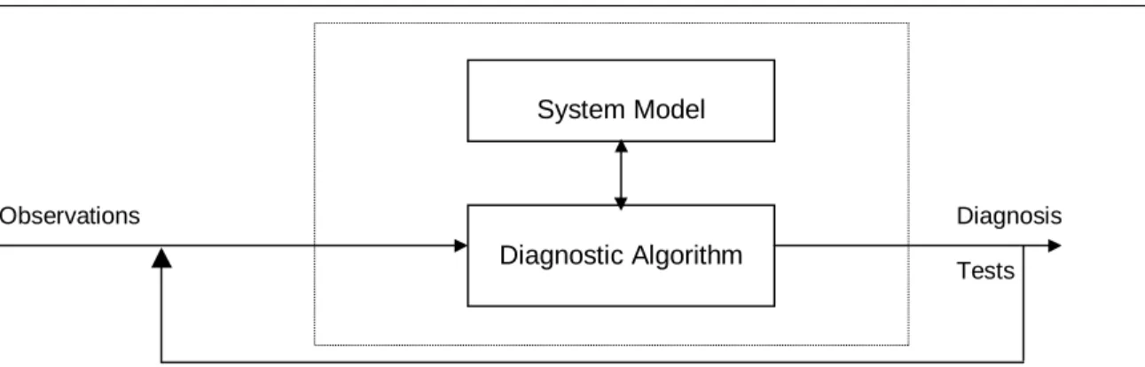
What can be done to handle these problems? The fundamentally different model-based diagnosis (MBD)

approach attempts to work out the diagnosis from a model of the normal behaviour of the system, rather

than work with an exhaustive list of faults and methods to diagnose each of them. It proposes a separation

of the diagnostic knowledge and the diagnostic procedure (figure 1). The diagnostic procedure is general

enough so that it can systematically analyze the given model (of any system) for generating diagnoses. Like

a human expert, the MBD approach attempts to reason from the model of the normal (or expected)

behaviour to work out all possible diagnoses that can “explain” the observations; for this reason MBD is also

called deep-knowledge diagnosis or diagnosis from first principles.

MBD has been used for diagnosis in a variety of practical domains like digital circuits, onboard aerospace

systems, automobile systems etc. The MBD approach is also a hot research sub-field, in particular to extend

its applicability to more complex systems represented in a variety of notations for specifying system models.

The MBD approach can be specialised to work with a number of mathematical or textual notations to

express and analyse models of systems. We focus on functional models of systems expressed using the

propositional logic. We then discuss a particular approach to MBD, called consistency-based diagnosis

(CBD), which relies on the notion of logical consistency. To be sure, propositional logic is simple and not

very expressive; e.g., it prohibits a proper modeling of dynamic systems having time-evolving inputs and

outputs (e.g., process control systems). However, it is adequate to model important aspects of static

systems like digital circuits. Note that the original papers in CBD, e.g., [1], do not presume any particular

logic; e.g., CBD can work with predicate logic or Horn clause logic as in the programming language Prolog.

Propositional Logic

A proposition is an atomic symbol (without any internal structure) that stands for a declarative statement

that can be true or false. Let PROP denote the set of propositions. Propositional logic provides the logical

also be defined. ¬ is a unary connective and the others are binary connectives. A formula is a string of

symbols constructed from propositions in PROP and the logical connectives; e.g., p → (q → (¬r)) and (p ∧

¬q) → r. An interpretation is a function I:PROP→{true, false} that associates a Boolean truth-value with each proposition in PROP. Truth-value TV(F) of a formula F is computed by combining the truth-values of its

sub-formulae, according to the truth-table in Figure 2.

For example, the formulae p → p and p ∨¬p are both true under all possible interpretations (i.e., p = true or

p = false); such a formula is called a tautology or validity. The formula p ∧¬p is not true (i.e., it is always

false) under any possible interpretation; such a formula is called unsatisfiable or contradiction. A formula

like p → q evaluates to true in at least one interpretation; such a formula is called consistent or satisfiable

and the corresponding interpretation is called a model for F. Given a formula F, checking whether F is

satisfiable is called the satisfiability problem. There is no known efficient (i.e., polynomial time) algorithm

to solve this problem that works for any arbitrary formula F in propositional logic.

Checking Satisfiability

A literal is a proposition or it negation; e.g., p and ¬q. A clause is a disjunction (∨) of zero or more literals;

e.g., p ∨¬q. A unit clause is the clause containing exactly one literal; e.g., ¬p. The empty clause, denoted

, is the clause that contains no literals; it is unsatisfiable. A formula F is said to be in conjunctive normal

form (CNF) if F has the form F1∧ F2∧ … ∧ Fn, where each Fi is a disjunction of literals; e.g., (p ∨¬q) ∧ (r ∨

s). There are efficient algorithms to transform any given formula in propositional logic into an equivalent

formula in CNF. We represent a formula F in CNF by the set {F1, F2, …, Fn}.

Figure 3 shows the basic Davis-Putnam algorithm [3] for checking the satisfiability of a propositional formula

in CNF. The unit subsumption rule is as follows. If there is a unit clause L in S, obtain S’ from S by

deleting those clauses in S containing L; if S’ is empty, then S is satisfiable. The unit resolution rule is as

follows. Obtain a set S’’ from S’ by deleting ¬L from every clause in which it occurs; S’’ is unsatisfiable if and

only if S’ is. Note that if ¬L is a unit clause, then it becomes when ¬L is deleted from it. These rules are

based on the facts that A ∧ (A ∨ B) is equivalent to A and A ∧ (¬A ∨ B) is equivalent to A ∧ B.

It is easy to verify, using the algorithm in Figure 3, that the set {p ∨ q ∨¬r, p ∨¬q, ¬p, r, u} is unsatisfiable,

the set {p ∨ q, ¬q, ¬p ∨ q ∨¬r} is satisfiable and the set {p ∨¬q, ¬p ∨ q, q ∨¬r, ¬q ∨¬r} is satisfiable.

We could also add the tautology rule to the algorithm: delete all clauses from S that are tautologies; the

remaining set is unsatisfiable if and only if S is. We could also add the pure literal rule, which is as follows.

A literal L is pure in S if the literal ¬L does not appear in any clause in S. If a literal L is pure in S, delete all clauses in S which contain L. The remaining set S’ is unsatisfiable if and only if S is.

System Models in Propositional Logic

Propositional logic can be used to model (nothing to do with a model as an interpretation which makes a

∧ ... ∧ Fn. A system description is a tuple (SD, COMPONENTS) where SD is a set of formulae in

propositional logic, constructed over the set PROP of propositions and COMPONENTS is a subset of PROP

which corresponds to a component in the system. Since each component is a proposition, we adopt the

convention that a truth-value of true (respectively false) for a component corresponds to a normally

functioning (respectively faulty) component. Figure 4 shows a simple digital circuit for a 3-bit adder [1] and

figure 5 shows a model in propositional logic for this circuit.

An observation of a system is a set OBS of formulae over PROP. In the normal system behaviour, all

components are non-faulty; this is expressed as a logical condition that SD ∪ OBS ∪ {c | c ∈

COMPONENTS} is consistent (i.e., satisfiable). However, if SD ∪ OBS ∪ {c | c ∈ COMPONENTS} is not consistent, then we need to perform a diagnosis i.e., identify the subset of faulty components that caused

the observation.

Formally, a minimal subset ∆ ⊆ COMPONENTS is a diagnosis if SD ∪ OBS ∪ { ¬d | d ∈∆} ∪ {c | c ∈

COMPONENTS - ∆} is consistent; ∆ is minimal in the sense that no proper subset of ∆ is itself a diagnosis.

In the adder example, an observation may consists of OBS = {in1, ¬in2, in3, out1, ¬out2} (i.e., in1=1, in2=0,

in3=1, out1=1, out2=0). Clearly, the adder is faulty; the expected output is out1=0 and out2=1. The

diagnosis task now is to identify which of the 5 components from the set COMPONENTS = {x1, x2, a1, a2,

o1} are faulty i.e., whose faulty behaviour can explain this observation. For the above example, there are

three diagnoses: ∆1 = {x1}, ∆2 = {x2, a2}, ∆3 = {x2, o1}. It is easy to check that each of these is indeed a

diagnosis; e.g., to check whether {x2, a2} is a diagnosis, one can verify that SD ∪ OBS ∪ {¬x2, ¬a2} ∪ {x1,

a1, o1} is consistent.

The central question in consistency-based diagnosis is how to systematically identify all possible diagnoses.

Consistency-based Diagnosis

The fundamental result of consistency-based diagnosis consists of a characterization of the faulty

components. For this purpose, we need the concepts of conflict sets, hitting sets and an HS-tree.

A conflict set for (SD, COMPONENTS, OBS) is a set {c1, c2, ..., ck} ⊆ COMPONENTS such that SD ∪ OBS

∪ { ¬c1, ¬c2, ..., ¬ck} is inconsistent. A conflict set for (SD, COMPONENTS, OBS) is minimal if no proper

subset of it is itself a conflict set for (SD, COMPONENTS, OBS). Intuitively, a conflict set (minimal or

otherwise) consists of those components at least one of which is definitely faulty.

Let C be a collection of sets. A hitting set for C is a set H of elements such that every element in H belongs

to at least one set S in C and H ∩ S ≠∅ for every set S in C. A hitting set for C is minimal if no proper

subset of H is itself a hitting set for C. For example,

The central characterization of a diagnosis is given by the following result. ∆ ⊆ COMPONENTS is a

diagnosis for (SD, COMPONENTS, OBS) iff ∆ is a minimal hitting set for the collection C of conflict sets for

(SD, COMPONENTS, OBS). For the adder, there are two minimal conflict sets {x1, x2} and {x1, a2, o1}. This

is because SD ∪ OBS ∪ {¬x1, ¬x2} is inconsistent and SD ∪ OBS ∪ {¬x1, ¬a2, ¬o1} is inconsistent. There

are three diagnoses, given by the minimal hitting sets for C = { {x1, x2}, {x1, a2, o1} }: ∆1 = {x1}, ∆2 = {x2,

a2}, ∆3 = {x2, o1}.

Let F be a collection of sets. An HS-Tree is an edge-labeled and node-labeled tree iff it is the smallest tree

with the following properties: (1) Its root is labeled by √ if F is empty. Otherwise it is labeled by an arbitrary

set of F. (2) If n is a node of G then define H(n) to be the set of edge labels on the path from the root to n. If

n is labeled by √ then it has no successor nodes. If n is labeled by a set Σ in F, then for each σ in Σ, n has a

successor node nσ, joined to n by an edge labeled by σ. The label for nσ is a set S in F such that S ∩ H(nσ) =

∅ if such a set exists; otherwise, nσ is labeled by √.

An HS-Tree has the following properties: (1) If n is a node of the HS-tree labeled by √, then H(n) is a hitting

set for F; and (2) each minimal hitting set for F is H(n) for some node n of the HS-tree such that n is labeled

by √. An HS-tree does not include all hitting sets for F but is does include all minimum hitting sets for F.

The essential idea behind Reiter’s algorithm [1] for computing all diagnoses for (SD, COMPONENTS, OBS)

is to treat F as the set of all conflict sets for (SD, COMPONENTS, OBS) and to construct an HS-tree to

generate all minimal hitting sets of F. F will not be explicitly available. We assume that a conflict-set

generator function GetConflictSet(SD,COMPONENTS,OBS) is available to generate a conflict set whenever

required. In this paper, we do not develop an algorithm for this function; it is not very complex for

propositional logic. Computing a conflict set is a very time-consuming operation and Reiter’s algorithm

attempts to minimize the number of times this generator is called.

(1) Generate the HS-Tree T in the breadth-first order, generating nodes at any fixed level in the tree from

the left to right order.

(2) Reusing node labels: If n is labeled by a set S in F and if n’ is a node such that H(n’) ∩ S = ∅ then label

n’ also by S. We indicate that the label of n’ is a reused label by underlining it in the tree. Computing

label(n’) does not require a call to the function GetConflictSet().

(3) Tree Pruning:

(i) If a node n is labeled by √ and a node n’ is such that H(n) ⊆ H(n’) then close n’ i.e., do not compute a label for n’ and do not generate any successors for n’.

(ii) If node n has been generated (but not labeled by √) and node n’ is such that H(n’) = H(n) then

close n’. We indicate a closed node in the HE-tree by marking it with ×.

(iii) If nodes n and n’ have been respectively labeled by sets S and S’ of F and if S’ is a proper

subset of S then for each α∈ S – S’ mark as redundant the edge from node n labeled α. A redundant edge, together with the sub-tree beneath it, may be removed from the HS-tree. A

As a last heuristic to improve the efficiency, whenever a node n in the tree needs a conflict set as a node

label, we call GetConflictSet(SD, COMPONENTS – H(n), OBS) rather than GetConflictSet(SD,

COMPONENTS, OBS). Such a call is guaranteed to return a set S such that S ∩ H(n) = ∅, if it exists.

Example

We come back to the adder example in Figures 4 and 5 and show how the algorithm works (see Figure 6

[1]). Suppose the first call to GetConflictSet(SD, {x1,x2,a1,a2,o1},OBS) yields the set {x1,x2}; this is the label

of the root. This generates two nodes n1, n2 on the next level where the edges from the root to them are

labeled by x1 and x2 respectively. Node n1 is labeled by the call GetConflictSet(SD, {x1,x2,a1,a2,o1} –

H(n1),OBS) = GetConflictSet(SD, {x2,a1,a2,o1},OBS) which returns √, since SD ∪ OBS ∪ { ¬x2, ¬a1, ¬a2,

¬o1} is consistent. Node n2 is labeled by the call GetConflictSet(SD, {x1,a1,a2,o1},OBS); suppose it returns {x1, a2, o1}. Node n3 is marked closed because of rule 3.(i) i.e., since there is a node n1 marked by √ such

that H(n1) = {x1} is a subset of H(n3) = {x1,X2}. Node n4 is labeled by the call GetConflictSet(SD,

{x1,a1,o1},OBS) which returns √ since SD ∪ OBS ∪ { ¬x1, ¬a1, ¬o1} is consistent.Similarly, the node n5 is

labeled √ by a call to GetConflictSet(SD, {x1,a1,a2},OBS). The set of all diagnoses is read from the tree of Figure 6 as {{x1}, {x2,a2}, {x2,o1}}. This particular HS-tree required 5 calls to the GetConflictSet() function. A

different implementation for this function may yield different conflict sets in subsequent calls (see figure 7).

Note that since the algorithm constructs the HS-tree in a breadth-first manner, it generates diagnoses in

increasing order of cardinality (number of faulty components).

Conclusion

The consistency-based diagnosis systematically works out the set of all possible diagnoses by reasoning

from a logical model of the normal behaviour of the system. In CBD, the model of a system is a set of

formulae in some mathematical logic and a diagnosis is a set of faulty components in the system, which

“explains” the observations by means of the notion of logical consistency. CBD is a fundamental and robust

approach to systematic diagnosis (as opposed to heuristic diagnosis). It diagnostic procedure is independent

to any changes in the system model. In this article, we discussed a specialised version of CBD where a

model and an observation both consist of a set of formulae in propositional logic and the components are a

set of propositions. CBD has been applied in a variety of interesting practical domains.

Acknowledgements

I sincerely appreciate the support and encouragement of Prof. Mathai Joseph. I also wish to thank Dr.

Manasee Palshikar for her confidence and perseverance in spite many serious obstacles.

References

[1] Reiter R.; (1987). A Theory of Diagnosis from First Principles. Artificial Intelligence, 32(1):57-95, 1987.

Proposed the CBD approach and the basic reference for this article.

[2] Hamscher W., Console L. and de Kleer J. (1992). Readings in Model-based Diagnosis, Morgan

Kaufmann, 1992. A collection of important papers in model-based diagnosis. Also includes a paper by

[3] Zhang H., Stickel M.; (2000). Implementing the Davis-Putnam Method, Journal of Automated Reasoning

24(1-2), Feb., 2000, pp. 277-296. The issue also contains articles defining the state of the art about the

SAT problem in propositional logic.

[4] Palshikar G. K., Khemani D. (1999), Diagnosing Dynamic Systems using Trace Patterns, Pattern

Recognition Letters, vol. 20, no. 7, July 1999. In this work, we used context-free grammar to model a

dynamic system and an observation was a string over an alphabet. The notion of logical derivations was

used to identify non-terminals, corresponding to faulty behavioural components.

Observations Diagnosis

Tests

Figure 1. Model based diagnosis has a general-purpose diagnostic procedure that works on a class of system models.

p q ¬p p ∧ q p ∨ q p → q p ↔ q p ⊕ q

true true false true true true true false true false false false true false false true false true true false true true false true false false true false false true true false

Figure 2. Truth-table to compute the truth-value of a formula.

Algorithm Satisfiable

Input clause set S Return Boolean

repeat

for each unit clause L in S do

delete from S every clause containing L // unit subsumption delete ¬L from every clause of S in which it occurs // unit resolution

end for

if S is empty then return TRUE else return FALSE endif; until no further changes result in S

// splitting

if Satisfiable(S ∪ {L}) then return TRUE

else if Satisfiable(S ∪ {¬L}) then return TRUE

else return FALSE endif

end

Figure 3. The Davis-Putnam procedure for checking whether a given formula in CNF is satisfiable [3].

System Model

in1

in2 a out1

in3

b

out2 c

x1, x2: XOR-gates a1,a2: AND-gates o1: OR-gate

in1, in2, in3: inputs out1, out2: outputs a, b, c: intermediate values

in1 in2 in3 out1 out2

0 0 0 0 0

0 0 1 1 0

0 1 0 1 0

0 1 1 0 1

1 0 0 1 0

1 0 1 0 1

1 1 0 0 1

1 1 1 1 1

Figure 4. A simple digital circuit [1] and a truth-table for its functionality

PROP = { x1, x2, a1, a2, o1, a, b, c, in1, in2, in3, out1, out2}

COMPONENTS = {x1, x2, a1, a2, o1}

SD = { x1 → (a ↔ (in1 ⊕ in2)), a1 → (c ↔ (in1 ∧ in2)), a2 → (b ↔ (in3 ∧ a)), x2 → (out1 ↔ (a ⊕ in3)), o1 → (out2 ↔ (b ∨ c)) }

The propositions {x1, x2, a1, a2, o1} correspond to the components in the circuit. The value true for a component indicates that the component is normal and a value false indicates that it is faulty.

Figure 5. A specification of the circuit in Figure 4 in propositional logic.

{x1,x2}

x1 x2

n1 √ {x1,a2,o1} n2

x1 o1 a2

n3 √ n4 √ n5 √

Figure 6. Pruned HS-tree for the adder example [1].

o1

x1

a2

x2

{x1,a1,a2,o1}

x1 )( a2 o1

√ {x1,x2} {x1,x2} {x1,x2}

x1 x2 x1 x2 x1 x2

× {x1,a2,o1} × √ × √