Counting points on K3 surfaces and other arithmetic-geometric objects

(1)

Cover Page

The handle

http://hdl.handle.net/1887/67532

holds various files of this Leiden University

dissertation.

Author: Visse, H.D.

(2)

Counting points on K3 surfaces and other arithmetic-geometric objects

Proefschrift

ter verkrijging van

de graad van Doctor aan de Universiteit Leiden, op gezag van Rector Magnificus prof.mr. C.J.J.M. Stolker,

volgens besluit van het College voor Promoties te verdedigen op dinsdag 18 december 2018

klokke 10 uur

door

Hendrik Dick Visse

(3)

promotor: dr. Ronald van Luijk promotor: prof.dr. Peter Stevenhagen Samenstelling van de promotiecommissie:

prof.dr. Aad van der Vaart (voorzitter; Universiteit Leiden) prof.dr. Bart de Smit (secretaris; Universiteit Leiden) prof.dr. Tim Browning (IST Austria / University of Bristol) dr. Damaris Schindler (Universiteit Utrecht)

dr. Arne Smeets (Radboud Universiteit Nijmegen)

(4)

Nothing will come of nothing

(5)

(6)

Introduction

O, for a muse of fire, that would ascend The brightest heaven of invention

Chorus,_{Henry V}, Prologue, lines 1-2

This thesis deals with three questions from arithmetic geometry. Even though it seems difficult to indicate one overarching topic, there do exist links between every pair of questions. Chapters 2 and 3 both deal with counting rational points, Chapters 2 and 4 are about K3 surfaces, and Chapters 3 and 4 both involve the concept of local solubility and obstruc-tions to global solubility.

In Chapter 1 we give some necessary background from geometry and num-ber theory that will allow us to study the topics in the later chapters. In particular, we give a quick treatment of the circle method, which is com-monly used to address counting questions from geometry. When studying a polynomialF ∈_Z[X1, . . . , Xn], then the integral

Z 1

0

exp(2πiαF(x))dα

tests if F has a zero at some point x ∈ Zn. Indeed, since F(x) is an

integer, the integral evaluates to 0 unless F(x) = 0 holds, in which case the integral equals 1. When for some bound B, we sum such integrals over all x ∈ (Z∩[−B, B])n, we may switch the order of the sum and

the integral. The circle method describes a quite general way in which this integral can be approximated well enough so that we get valuable information out of it for large B. Moreover, this process generalizes to multiple polynomials. For now, it suffices to know that the main term will be a product of an integral (which should be easier to compute) and a series.

(9)

INTRODUCTION

to bounded height. If x = (x0 : . . . : xn) ∈ Pn(Q) is any point, we

may arrange its coefficients so that each of the xi is an integer, and the

(n+ 1)-tuple has trivial greatest common divisor. If we do that, then we callH(x) = maxi|xi|the height of the pointx. A useful property is that

for any given bound B, there are only finitely many points in Pn(Q) that

have height at mostB. The same is true for any subvariety ofPn_Q. Hence,

for any given subvariety, we may count this number N(B) of points for varying B. In the case of Fano varieties, Manin stated a rather general conjecture for the shape of N(B), involving some geometric invariants. In particular, Manin’s conjecture asks us to restrict ourselves to open subsets since there might exist so-called accumulating subvarieties. These may contain ‘too many’ rational points and we should ignore those. Many examples of Fano varieties have been studied in the literature, and at least for surfaces there are many examples where N(B) involves a power of B

and a power of log(B). The exponent of the logarithm is ρ−1, where ρ

is the rank of the Picard group of the variety.

Leaving the world of Fano varieties, we study diagonal quartic surfaces, which are examples of K3 surfaces, and we employ the circle method to count zeroes of the defining equation. Experts will immediately recognize that in this case the emergent error terms will exceed the desired main term. We focus on the main term and we speculate that there should be a connection between the error terms and accumulating subvarieties on the surface. Such behaviour has been observed in the literature for other types of varieties, but a detailed treatment supporting such speculation seems out of reach of our methods. The main result of this chapter gives heuristic support for hitherto unexplained data obtained in computer ex-periments by van Luijk some years ago. In particular we find that no power of B occurs and in contrast to the Fano varieties discussed above, that the power of log(B) ought to beρinstead. Apart from this result, the approach to obtain these heuristics could be viewed as the main contribu-tion of this chapter: we use averaging results of multiplicative funccontribu-tions to study the series coming out of the circle method, and we exploit the Tate conjecture to determine the exponent of the logarithm via the L-function of the surface. This givesρ−1 factors of log(B), while the last logarithm is obtained from the remaining factor that comes in the form of an integral.

(10)

INTRODUCTION

precisely, he studied the number of rational points in the base up to a bounded height, say B, such that the fibres over these points contain a rational point themselves. Serre was only able to prove upper bounds, but for his specific examples it has since been shown that these upper bounds are in fact asymptotically correct. In recent years more examples of fibrations, not necessarily conic bundles, have been studied. Most notably, Loughran and Smeets have provided a framework into which results in this area should fit. Complete examples in the literature are rare, and our contribution lies in giving a wide class of conic bundles for which we can not only prove asymptotic results, but where we are also able to study the leading constant of such asymptotics. In particular, we look at bundles that can locally be described as follows. We take two polynomials

f1 and f2 in n variables and of even degree d, subject to some more

conditions that are outlined in Chapter 3. Now consider the variety B

defined by f2(t1, . . . , tn) = 0 as a subvariety of Pn_Q−1. Over the affine

patch where we take ti = 1, we define a conic bundle

x2+y2=f1(t1, . . . , ti−1,1, ti+1, . . . , tn)z2,

f2(t1, . . . , ti−1,1, ti+1, . . . , tn) = 0.

These bundles glue together into a conic bundle φ : X → B. Now let

N(B) be the number of rational points ofBup to heightB, the fibre over which has a rational point itself. Then we prove that there is a constant

cφ such that we have

N(B) =cφ

Bn−d

(logB)1/2

up to an error term with a logarithmic exponent slightly bigger than 1/2. Moreover, our methods allow us to prove a Hasse principle on smooth fibres. To obtain our results, we use the circle method together with sieving techniques to study the series that appears. The conditions on the fibre in order for it to contain rational points appear through an indicator function detecting everywhere local solubility. Since our fibres are conics and therefore themselves satisfy the Hasse principle, this guarantees global solubility. Considerable effort goes into writing the leading constantcφas

a product of recognizable factors, and we indicate how this fits conjectural expectations first described by Loughran.

(11)

INTRODUCTION

Victoria Cantoral-Farf´an, Yunqing Tang, and Sho Tanimoto, we study Brauer groups of Kummer surfaces. In particular, by a celebrated result of Skorobogatov and Zarhin we know that for any K3 surface over the field of rational numbers, its Brauer group (modulo constants) is finite. Our work gives explicit upper bounds for the size that this group may attain, at least when dealing with Kummer surfaces. For an abelian surfaceAover a number fieldk, with Kummer surfaceX, it is known that Br(A) and Br(X) are isomorphic as Galois modules, and we will bound the transcendental Brauer group Br(X)/Br1(X) as a subgroup of Br(X)Γ, where Γ denotes

the absolute Galois group ofk.

The proof of Skorobogatov and Zarhin’s result relies on an exact sequence of cohomology groups, namely

0→ NS(A)/`nΓ→fn H_et_´2 (A, µ`n)Γ →Br(A)Γ_`n →

→H1(Γ,NS(A)/`n)→gn H1(Γ,H2_´_et(A, µ`n)),

whereA is an abelian surface over a number fieldk,`is a prime number, and the subscript `n indicates`n-torsion. We use this exact sequence and we study the cokernel of fn and the kernel of gn. Bounds on their sizes

imply bounds on the size of Br(X)Γ_`n, and we provide bounds independent of n. There are only finitely many ` for which such bounds are non-trivial, so we should also bound the size of such `. This last point in particular relies on effective versions of Faltings’ finiteness theorem for abelian varieties.

Although the existence of upper bounds like ours is not new, our methods have the advantage of being more explicit than those that were already known, especially for Kummer surfaces of minimal Picard rank. In par-ticular, if one is given a curve C of genus 2 over a number field k, for which the Jacobian Jac(C) has Picard rank 1 and Faltings height h, let

δ denote the discriminant of NS(X), where X is the Kummer surface of Jac(C). In order to obtain an upper bound for the transcendental part # Br(X)/Br1(X), one needs only apply our formula with inputs [k:Q],

h, andδ. Moreover, we prove that the algebraic part Br1(X)/Br0(X) has

order at most 2. Although our bounds are explicit, they are unlikely to be sharp. We compute the example of the curve C given by

y2=x6+x3+x+ 1.

(12)

Chapter 1

Background

Though this be madness, yet there is a method in’t

Polonius,_Hamlet, Scene 2.2, line 207

1.1 Notation

Throughout this thesis, we will often use the font x as short-hand for either a tuple (x1, . . . , xn) or a collection of variablesxi where the range

of iis to be understood.

For functions f, g:R→Rwe write

• f(x) =o(g(x)) if limx→∞ f_g(₍x_x)₎ = 0;

• f(x)∼g(x) if either f(x) =g(x) = 0 holds for all sufficiently large

x, or limx→∞ f_g₍(x_x₎) = 1;

Somewhat differently, given a subsetR⊂_Rm+n_{and a function}_f _:_R_→

R,

we write

f(s1, . . . , sm, x1, . . . , xn) =Os1,...,sm(g(s1, . . . , sm, x1, . . . , xn)) for some functiong:R →_R≥0, or equivalently

f(x1, . . . , xn)s1,...,sm g(s1, . . . , sm, x1, . . . , xn),

if there exists a non-negative valued functionC whose domain is the pro-jection of R onto Rm given by its first m coordinates, such that for all

(s1, . . . , sm, x1, . . . , xn)∈R we have

(13)

1.2. GEOMETRY AND RATIONAL POINTS

We will often think abouts1, . . . , sm as parameters andx1, . . . , xnas

vari-ables. Hence by a slight abuse of language, any suchCis called an implied constant.

When we write f(s,x) =h(s,x) +Os(g(s,x)), then this should be inter-preted to mean f(s,x)−h(s,x) =Os(g(s,x)).

Furthermore, we will write f(s,x) = Θs(g(s,x)) or f(s,x) s g(s,x) if both f(s,x) = Os(g(s,x)) and g(s,x) = Os(f(s,x)) hold, possibly with different implied constants.

One should note that this notationO( ) differs in use from that of Landau or Bourbaki, but it is in line with the use in standard references like [IK04] or [MV07] and many papers in analytic number theory.

The notation 1A for some conditionAwill be used for the indicator

sym-bol, that is 1A = 1 if and only if the condition A holds, and 1A = 0

otherwise.

1.2 Geometry and rational points

Since this thesis deals with number theory in a geometric context, we will need to recall a few concepts from geometry.

Definition 1.2.1. A variety is a separable scheme of finite type over a field. We call a variety nice if it is smooth, projective, and geometrically integral over its base field.

Definition 1.2.2. Acurve is a variety of pure dimension 1. A surface is a variety of pure dimension 2.

Definition 1.2.3. If X is a nice variety and D and D0 are two effective divisors, then we say that Dand D0 are linearly equivalent if there is an element f of the function field satisfying divf = D−D0. The Picard group PicX is the free abelian group of divisors on X divided out by linear equivalence.

In the definition above, the element f may be viewed as a rational map

X →_P1_{, which will make}_D_and_D0 _{fibres over two closed points (namely}

0 and∞). By applying an automorphism ofP1, we may move 0 and∞ to

(14)

Definition 1.2.4. Let X be a nice variety with two effective divisors D and D0. We call D and D0 pre-algebraically equivalent if there exists a smooth curve C, two points x and x0 on C, an effective divisor D on

X×C with a flat morphism f :D → C such that we have D =f−1(x) and D0 = f−1(x0). The equivalence relation generated by pre-algebraic equivalence is called algebraic equivalence. The group of divisors divided out by algebraic equivalence is the N´eron-Severi group of X, denoted NSX.

Remark1.2.5. Both PicX and NSX are abelian groups by construction.

IfXis a nice surface, then one can define a symmetric bilinear intersection pairing ( · ) : PicX ×PicX → Z which further induces a pairing on

NSX. The N´eron-Severi group of a nice surface is finitely generated and consequently has finite rank. Thus the pairing turns NSX into a lattice.

IfX is a nice surface overC, the N´eron-Severi lattice NSX injects

canon-ically into H2(X,Z), which is a lattice by the cup product pairing. The

lattice structures are compatible.

Definition 1.2.6. For a nice surface X over C, we call the orthogonal

complement of NSX in H2(X,Z) thetranscendental lattice ofX, denoted

T(X).

Definition 1.2.7. For a nice surface X, we call the rank of its N´ eron-Severi lattice its Picard rank or sometimes N´eron–Severi rank. We often denote this number by ρ(X) or justρ.

For a nice surfaceX, one may take a further quotient of PicXby numerical equivalence, defined as follows.

Definition 1.2.8. For a nice surface X, two line bundles L, L0 ∈ PicX are called numerically equivalent if for every line bundleL00 we have the equality (L·L00) = (L0·L00). The quotient of PicXby numerical equivalence is denoted NumX.

Linear equivalence implies algebraic equivalence, which in its turn implies numerical equivalence, so by taking repeated quotients there are natural surjections

(15)

1.2.1 K3 surfaces

Definition 1.2.9. A K3 surface is a nice surface X satisfying the follow-ing two properties:

• The canonical bundleωX is isomorphic toOX.

• The cohomology group H1(X,O_X) is trivial.

Example 1.2.10. We list a few basic examples of K3 surfaces:

• quartic surfaces in P3,

• double covers ofP2 branched along a smooth sextic curve,

• the minimal resolution of the quotient of an abelian surface by the action of -1; these are calledKummer surfaces.

Proposition 1.2.11. If X is a K3 surface, then the mapsPicX→NSX

and NSX → NumX are isomorphisms and the intersection pairing on

PicX is even and non-degenerate and has signature (1, ρ(X)−1).

Proof. This is [Huy16, Prop 1.2.4]. The proof almost entirely relies on the Riemann–Roch formula for surfaces and the Hodge index theorem.

For a K3 surface X overC, the cohomology group H2(X,Z) has a Hodge

structure as H2(X,C)∼= H2,0⊕H1,1⊕H0,2, where we have written Hp,q for

Hq(X,Ωp_X/

C) and ΩX/C is the sheaf of K¨ahler differentials on X. These

summands have dimensions 1, 20, and 1 respectively. The Lefschetz (1,1)-theorem assures that under the canonical embedding NSX lands in H1,1∩H2(X,Z). Thus the Picard rank of a K3 surface over a field

of characteristic zero satisfies 1 ≤ ρ(X) ≤ 20. In positive characteristic higher Picard ranks may be achieved, however still no higher than 22.

1.2.2 Manin’s conjecture

Definition 1.2.12. Letx= (x0 :x1:. . .:xn)∈Pn(Q) be any point and

for all coordinates assume xi ∈ Z without loss of generality and further

assume gcd(x0, . . . , xn) = 1. Then theheight ofx is H(x) = maxi|xi|.

Given a projective varietyX overQand a very ample divisorDonX we

can embed X into somePn_Q usingD. This induces a height function as in

(16)

the specific set of global sections chosen to give the embedding. We write

HD for this height function.

Definition 1.2.13. Let U ⊂ X be an open subvariety of a variety X embedded in Pn_Q via a very ample divisor D. We write

NU,D(B) = #{x∈U(Q)|HD(x)≤B}.

Remark 1.2.14. The numberNU,D(B) is always finite. This is known as

the Northcott property of the height HD.

In the late 1980’s, Manin stated a conjecture, first recorded in [FMT89], concerning the heights of rational points of Fano varieties. It was later extended most notably by Batyrev and Manin [BM90] and Peyre [Pey95]. Manin’s original formulation is for Fano varieties. A smooth variety X is called Fano if its anticanonical divisor −K_X is ample.

Conjecture 1.2.15 (Manin). For any Fano variety X over Q of

Pi-card rank ρ and with very ample anticanonical divisor −KX, there exists

an open subvariety U ⊂ X and a non-negative constant cX such that as

B → ∞ the following holds:

NU,−KX(B)∼cXBlog(B)

ρ−1_.

Refinements of this conjecture allow one to go beyond the case of Fano varieties, at the cost of some precision. For example, we have the following conjecture from [BM90].

Conjecture 1.2.16 (Batyrev–Manin). For a K3 surfaceX over Q, take

ε ∈ R>0 and let D be a very ample divisor on X. Then there exists a

non-empty Zariski open subvarietyU(ε)⊂X such that forB ≥1 we have NU(ε),D(B) =Oε(Bε).

(17)

In all of these conjectures, one is forced to take an open U ⊂ X rather than state the conjecture just for X itself since X may contain so-called accumulating subvarieties. These are subvarieties ofXthat upon counting their rational points up to height B would give an asymptotic that domi-nates the expected main term in the Manin conjectures. It can be shown that embedded rational curves of degree d asymptotically contribute a constant multiple ofB2/dto the counting, so for Fano varieties it is neces-sary to exclude embedded lines, by which we merely mean the casesd= 1. However, there are examples where leaving out a finite number of accu-mulating subvarieties is not enough, see for example the counterexample by Batyrev and Tschinkel in [BT96], where infinitely many subvarieties give the ‘correct’ exponent of B, but an exponent of logB that is too high. It is a topic of active research to find the correct modification of the conjectures to accommodate for these defects, see for example [Rud14], [Pey17], [Pey18], [LST18], or the overview article [LT18].

In the case of K3 surfaces, where the expected exponent of B is 0, the problems are even worse. Not only do embedded rational curves of any degree provide problems, so may embedded elliptic curves. For an elliptic curve E of Mordell–Weil rank rE, it is a classical result by N´eron that

there is a contantc validating

NE(B)∼c(logB)rE/2,

see for example [Ser97, §4.5] where the constant c is also given. Hence if our heuristic is correct, every elliptic curve satisfyingrE >2ρ will need to

be removed before counting rational points on the remainder. Here one quickly encounters an active research problem of an entirely different na-ture: since any elliptic curve on a K3 surface provides an elliptic fibration (this may be proven using the Riemann–Roch formula for surfaces), one is directed to the question how Mordell–Weil ranks vary in families of elliptic curves. However interesting these problems may be, we will not consider them in this thesis, and we leave the discussion here only for the sake of the interested reader.

One cannot discuss Conjecture 1.2.15 without mentioning the conjec-tural refinement obtained by Peyre [Pey95], with a small modification by Batyrev and Tschinkel [BT95]. In these papers, a geometric interpre-tation is given to the constantcX: one should expect this constant to have

the shape

cX =α(X)β(X) lim s→1(s−1)

ρ_L₍_s₎Y

v

τv

Lv(1)

(18)

where α(X) measures the volume of some region in the cone spanned by effective divisors in the real vector space NS(X)⊗_R; the factor β(X) equals the order of the finite group H1(Gal(Q/Q),PicX); for each place

v of Q the τv are Tamagawa numbers, or otherwise put they are v-adic

measures of the ad`elic points ofX; the numbersLv(1) are factors making

the infinite product converge; and the limit balances out these convergence factors.

We will not include a detailed treatment of this conjectural constant, but while we were thinking about possible adaptations to the case of K3 sur-faces, a point of confusion came up in several conversations with other researchers. We do want to address this quickly. The cohomology group H1(Gal(Q/Q),PicX) may be recognized as the algebraic Brauer group

Br1(X)/Br(Q). For Fano varieties the algebraic part forms the entire

Brauer group: there are no transcendental elements. Passing to K3 sur-faces, transcendental elements may in fact exist, but it is known that the Brauer group is still finite. This was first proven in [SZ08], and it forms the basis for the work in Chapter 4. Based purely on this recognition one could guess that it is in fact # Br(X) that should replace β(X) in general. However, if one looks more closely at the available literature (for example in the very detailed paper by Salberger [Sal98]), one finds that H1(Gal(Q/Q),PicX) also parametrizes so-calleduniversal torsorsoverX,

which may be applied when counting rational points onX. The connection to the (algebraic) Brauer group seems to be merely coincidental. Based on conjectures about Brauer–Manin obstructions to weak approximation on Fano varieties, some researchers seem to believe that the factor β(X) should somehow measure the failure of weak approximation. Because the recognition of # Br1(X)/Br(Q) inβ(X) seems coincidental to us, we

be-lieve that such an interpretation falls in the realm of wishful thinking. One should however note that in uncharted terrain, wishful thinking may be a guiding principle, and one should try and avoid negativity.

(19)

the leading constant. Loughran discusses a theoretical framework in which one should place the leading constant for this problem, and we compare our findings to his framework in §3.5.4.

1.2.3 L-functions of varieties

We will first define the zeta function of varieties over finite fields, before moving on to characteristic zero.

Definition 1.2.17. LetXp be a nice variety defined overFp. One defines

thezeta function ofXp as

ζ(Xp, T) = exp

∞ X

m=1

#Xp(Fpm)

m T m

! .

IfX is a nice variety defined overQsuch thatX has a finite presentation

model X over Z, we write Xp for X ×SpecZSpecFp. The further base

change to Fq is denoted Xq and we write Xp for the base change to Fp.

As per usual we write S for the (finite) set of primes p where Xp is not

smooth.

There is a well-known connection between zeta functions of varieties and traces of Frobenius via the Lefschetz trace formula. For q a power of p, we write τq,i,`for tr Frobq|H´iet(Xp,Q`)

, (`6=p). TheFq-rational points

of Xp are the closed fixed points of Frobq :Xp → Xp, and the Lefschetz

trace formula gives

#Xp(Fq) =

2 dimX

X

i=0

(−1)iτq,i,`.

and this equality is independent of `.

If we denote the eigenvalues of Frobp on Hi´et(Xp,Q`) by αij, and writebi

for the dimension of H_´i_et(Xp,Q`), then by the Lefschetz trace formula we

(20)

ζ(Xp, T) =

2 dimX

Y

i=0

bi

Y

j=1

exp (−1)i

∞ X

m=1

αm_ijTm m

!

=

2 dimX

Y

i=0

bi

Y

j=1

exp (−1)i+1log(1−αijT)

=

2 dimX

Y

i=0

bi

Y

j=1

(1−αijT)(−1)

i+1

and hence

ζ(Xp, T) =

2 dimXp

Y

i=0

det 1−FrobpT |H´iet(Xp,Q`)

(−1)i+1

. (1.1)

So far, we have used the terminology of zeta functions, but from now on we want to switch over to the terminology of L-functions. In some sense there is no difference: theL-function of a variety in characteristicpis just its zeta function, but with the variable T replaced by p−s. For varieties overQas above we do this at every p-adic factor.

Definition 1.2.18. The L-function of X is defined via ζ(Xp, T) as

L(X, s) =Y

p /∈S

ζ(Xp, p−s),

where S is the set of bad primes.

Some authors prefer to extend the definition of L(X, s) to include factors for every prime p, rather than only those not inS. In that case one refers to (1.1) but instead lets 1−FrobpT act on the part of Hi´et(Xp,Q`) that is

fixed by the inertia group atp. Forp /∈S, this interia group acts trivially so there is no modification.

As for the zeta functions in (1.1), these L-functions break apart into fac-tors, one for each iin the range 0≤i≤2 dimX.

Definition 1.2.19. We will also write

L(Hi(X), s) =Y

p /∈S

det 1−Frobpp−s|Heti´ (Xp,Q`)

(−1)i+1

(21)

L-functions for K3 surfaces

If X is a K3 surface, the only non-trivial `-adic ´etale cohomology occurs at i= 0, i= 2, and i= 4. The factorL(H2(X), s) will be of importance in Chapter 2.

For K3 surfaces, we study theL(H2(X), s) somewhat further. In [PSD91], it is explained thatL(H2(X), s) breaks apart into two multiplicative parts: one part L0(H2(X), s) coming from the N´eron-Severi lattice (over the al-gebraic closure), and the other L00(H2(X), s) coming from the transcen-dental lattice. The first part itself breaks down as a product of shifted Riemann zeta functions ζ(s−1) and other similarly shifted Dirichlet L -series, coming from the Galois representation on the N´eron-Severi lattice. The multiplicity ofζ(s−1) that occurs is equal to the rank of NSX. In the number theory part of this chapter we will mention a well-known and important property of Dirichlet L-series, namely Theorem 1.3.39. In the currect context, this theorem shows that only the factors ζ(s−1) contribute to the pole ats= 2 and consequently that the rank of NSX is equal to the order of the pole of L0(H2(X), s) at s= 2. The same holds for the fullL(H2(X), s), provided that the factor L00(H2(X), s) is analytic at s = 2. For diagonal quartic surfaces in particular, this was already studied, yet not fully proven, in [PSD91]. Their results are a special case of the following general principle of modularity, which we will not define, but whose consequence will be useful.

Over some extension of the base field, every diagonal quartic surface is isomorphic to the Fermat quartic x4₁+x4₂+x4₃+x4₄ = 0. This surface is known to have maximal Picard rank 20 overQ. K3 surfaces with geometric

Picard rank 20 are called singular K3 surfaces where the word singular is not to be confused with the negation of non-singular or smooth. Livn´e proved the following important theorem.

Theorem1.2.20 (Livn´e). Every singular K3 surfacesX overQis

modu-lar. The 2-dimensional Galois representation defined by the transcendental latticeT(X) has an associated modular form that is a Hecke eigenform of weight 3 with complex multiplication by Q(p−disc(NSX)).

Proof. This is proven in [Liv95].

(22)

well-behaved in many regards. In particular we have the following theo-rem.

Theorem 1.2.21 (Hecke). The L-function L(f, s) of a modular form f

of weight k has a meromorphic continuation to the whole complex plane and satisfies a functional equation. Moreover, L(f, s) is entire if f is a holomorphic cusp form, and otherwise it has only a simple pole at s=k.

Proof. This is [IK04, Theorem 14.7].

Remark 1.2.22. None of this should come as a surprise. In his excel-lently written [Tat65], Tate repeats his conjecture that relates the Picard rank of a variety to the order of the accociated pole of L(H2(X), s). For K3 surfaces, the full Tate conjectures are now known through work of Andr´e [And96] and Tankeev [Tan88] in characteristic zero, in odd charac-teristic by work of many people, among them Nygaard and Ogus [NO85], Maulik [Mau14], Charles [Cha13], and Madapusi Pera [MP15], and finally in characteristic 2 by Kim and Madapusi Pera [KMP16].

In preparation of this thesis, a point of confusion came up relating to this. It may be useful to spend a few words in order to make sure that the reader does not fall victim to the same fate.

If Xp is a nice surface over Fp, then the Tate conjecture says that for

L(H2(Xp), s) the order of the pole at s= 1 equals the Picard rank of Xp.

Indeed, if the rank is ρ, then there will be at least ρ eigenvalues among the α2j that are exactly p. These correspond to the eigenvalues 1 on the

twisted cohomology group H2_´_et(Xp,Q`(1)). Conjecturally these are all of

them.

Now let X be a nice surface over Q with good reduction Xp at p. Then

the p-adic factor of L(H2(X), s) should have a pole of order ρ(Xp) at

(23)

1.3. NUMBER THEORY AND SOLVING EQUATIONS

Let us consider an easy example: X =Pn_Q. We have PicX∼=Z. It is not

difficult to derive L(H2(X), s) =ζ(s−1), where ζ denotes the Riemann zeta function. Indeed this function has a pole of order 1 at s = 2, and value −1

2 ats= 1.

1.3 Number theory and solving equations

In this section we will collect some results from number theory, in partic-ular we will mostly discuss the circle method, which is to be used to count rational or integral solutions to polynomial equations. Before we set off, we will mention a few results which will come up several times.

Theorem 1.3.1 (Abel’s summation formula). Let (an)n be a sequence of

complex numbers and let φ : R>0 → R be differentiable with continuous

derivative. For any x ∈ _R≥1, write A(x) = P₁≤n≤xan. Then for all

1≤y < x the following equation holds:

X

y<n≤x

anφ(n) =A(x)φ(x)−A(y)φ(y)−

Z x

y

A(t)φ0(t)dt.

Proof. This is [Apo76, Theorem 4.2].

We also record the famous Prime Number Theorem here, mostly because a high brow proof of it will be a guide for the methods in §2.2, but secon-darily also since its statement will briely occur in combination with Abel’s summation formula in that same section.

Theorem 1.3.2 (Prime Number Theorem). Let π(x) denote the number

of primes up to x. The function π(x) satisfies

π(x)∼ x

logx.

(24)

1.3.1 The circle method

In this subsection we give a treatment of the basics of the circle method. The reader wishing to learn more is adviced to read for example [Bro09], [Dav05], or [IK04]. The circle method was first developed by Hardy and Ramanujan to study partitions of numbers, and later adapted to study zeroes of polynomials over Z.

LetF(x)∈Z[x] be a homogeneous polynomial of degreedinnvariables.

The goal for which the circle method is commonly applied is to count integral zeroes ofF in some bounded boxB= [−B, B]n.

The starting point of the method is the following indicator integral, where x is an integer vector:

Z 1

0

e(αF(x)) dα=

(

1 if F(x) = 0,

0 otherwise,

where we have written e(z), and will continue to do so, when we mean exp(2πiz).

Definition 1.3.3. We write NF(B) for the number of integral zeroes of

F in the regionB.

By applying the above indicator integral, we have

NF(B) =

X

x∈_Zn_∩B

Z 1

0

e(αF(x)) dα

=

Z 1

0

X

x∈Zn∩B

e(αF(x)) dα.

Notice that switching the sum and the integral is allowed because the sum is over a finite set.

Without applying any machinery to study this integral expression, one may very intuitively guess that the number NF(B) should behave as

O Bn−dbecause of the following argument. When we varyxoverZn∩B,

(25)

applies, will indeed provide this exponentn−dofB, combined with more detailed information, such as additional logarithmic factors.

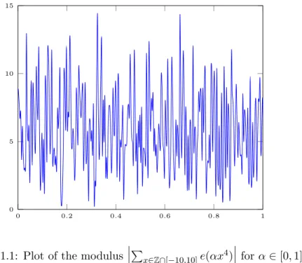
The method assumes that the main contributions to the integral occur around numbers α that are well approximated by rational numbers with small denominator, and according to this philosophy divides the range of integration up into segments centred around these well-approximable num-bers. Figure 1.1 shows a sketch of the modulus of P

x∈_Z∩[−10,10]e(αF(x))

for a simple polynomial F(x) =x4. Although the plot does not indicate whether this philosophy makes sense, at least it is clear that the value of the function shows quite erratic behaviour.

0 0.2 0.4 0.6 0.8 1

0 5 10 15

Figure 1.1: Plot of the modulus

P

x∈_Z∩[−10,10]e(αx4)

forα∈[0,1].

We let δ be a small parameter which will stay free to be chosen later and write Q=Bδ.

Definition 1.3.4. Fora, q∈Zcoprime satisfying 1≤a≤q ≤Q, we call

the interval Mq,a(δ) =

h

a q −B

−d+δ_,a q+B

−d+δi _the_{major arc centred at} a

q. We writeM(δ) for the union of major arcs andm(δ) = [0,1]\M(δ) for

(26)

Lemma 1.3.5. For δ < d₃ and B > 2 1

d−3δ _{different major arcs do not}

overlap.

Proof. This is [Bro09, Lemma 8.3] We take two centresa_q and a_q00 of different major arcs and consider the difference D:=|a

q− a0

q0|. Using a_q 6= a 0

q0 in the shape |aq0−a0q| ≥1, we findD ≥ _B12δ. On the other hand, the triangle inequality with a supposed midpoint in the intersection of these two major arcs shows D≤2B−d+δ_{. This is in contradiction with the quoted values}

forδ andB.

We now want to study the behaviour of the integrandP

x∈Zn∩Be(αF(x))

in a certain major arc Mq,a. We write α= a_q +θ and we split the

expo-nential. Realizing thatea_qF(x)as a function ofxis periodic moduloq, we find

X

x∈Zn∩B

e(αF(x)) = X u∈(Z/qZ)n



  

ea_qF(u) X

x∈Zn∩B

x≡u(modq)

e(θF(x))



  

. (1.2)

Definition 1.3.6. We write

I(t) =

Z

[−1,1]n

e(tF(x))dx.

Notice that the integral I(θ) only depends on F.

Lemma 1.3.7. For 1≤a≤q ≤B with gcd(a, q) = 1, and α = a_q +θ we

have

X

x∈Zn∩B

e(αF(x)) =

B q n   X

u∈(Z/qZ)n e

a qF(u)



·I(θBd)

+O

qBn−1(1 +|θ|Bd)

.

Proof. This is [Bro09, Lemma 8.2]. Its proof relies on showing that the ex-pressionP

x∈Zn∩B

x≡u(mod q)

(27)

This process can be applied for every major arc, or in other words for every 1≤q≤Qand everya∈(Z/qZ)×, provided Q≤B or equivalently

δ ≤1 hold. Changing variables within the integral over any major arc

Z B−d+δ

−B−d+δ

I(θBd)dθ=B−d Z Bδ

−Bδ

I(θ0)dθ0,

for sufficently small δ and large B, that is as in Lemma 1.3.5, we finally arrive at

NF(B) =Bn−dJ(Q) Q

X

q=1

1

qn

X

a∈(Z/qZ)× X

u∈(Z/qZ)n e

a qF(u)

+

Z

m X

x∈Zn∩B

e(αF(x)) dα+E

(1.3)

with

J(R) =

Z R

−R

I(θ)dθ=

Z R

−R

Z

[−1,1]n

e(θF(x))dxdθ,

and where the error E comes from integrating the error term in Lemma 1.3.7 over the range θ ∈(−B−d+δ_{, B}−d+δ_{) and afterwards summing over}

a∈(Z/qZ)× and 1≤q ≤Q=Bδ. It satisfies

E =O

Bn−1−d+5δ

.

Remark 1.3.8. In order to avoid the possibility of the error termE dom-inating, one should pick δ to satisfy δ < 1₅, rather than merely δ < d₃ as suggested by Lemma 1.3.5. From now on, we will always assume that the errorE is asymptotically small.

Definition 1.3.9. It is convenient to name some parts of the expression (1.3). We introduce the following notation:

• Sq,a =P_u∈(Z/qZ)ne

a qF(u)

,

• Sq =P_a∈(Z/qZ)×Sq,a,

• S(Q) =PQ

q=1q1nSq.

(28)

In many applications the singular integral converges for R → ∞, and therefore is approximated by the same integral but with the range of in-tegration stretched out to the whole real line.

Remark 1.3.10. In the application of Chapter 2, the singular integral actually does not converge.

People say that “the circle method works” when one can prove that the major arcs give the main contribution to NF(B) and the minor arcs give

an error term which is smaller, at least asymptotically. This usually needs

nto be rather big compared tod. A naive probabilistic reasoning indicates how big n should be compared to d. For fixed α ∈ m(δ) one may think that the values of e(αF(x)) will be randomly distributed over the unit circle when ranging over all x∈[−B, B]n∩_Zn_{. We are interested in their}

sum and the central limit theorem suggests that the absolute value of this sum will tend top#([−B, B]n_∩_Zn₎_∼₍₂_B₎n/2_{. On the other hand, the}

exponent of B appearing in equation (1.3), arising from the major arcs, is n−d as usually the singular integral and singular series converge for

Q→ ∞. Hence we expect to need n >2d variables for the circle method to work. In reality however, one often needs many more variables than suggested by this heuristic lower bound.

Lemma 1.3.11. As a function inq, the symbol Sq is multiplicative.

Proof. This proof is taken from [Dav05, Lemma 5.1], adapted to our sit-uation. If q1 and q2 are coprime, write q=q1q2 and

a≡a1q2+a2q1(modq) (1.4)

for anya∈(Z/qZ)×. It suffices to prove the validity ofSq,a=Sq1,a1Sq2,a2

since the Chinese Remainder Theorem gives a group isomorphism between (Z/qZ)× and (Z/q1Z)××(Z/q2Z)×, yielding

Sq=

X

a∈(Z/qZ)× Sq,a =



 X

a1∈(Z/q1Z)× Sq1,a1



 

 X

a2∈(Z/q2Z)× Sq2,a2



=Sq1Sq2.

Similarly, using the Chinese Remainder Theorem in its more general state-ment about the ringsZ/qZ∼=Z/q1Z×Z/q2Z, we may uniquely write any

u∈_Z/qZas

(29)

where no assumption of coprimality between the ui and qi is present. We

have

Sq,a =

X

u∈(Z/qZ)n e

a qF(u)

= X

u1∈(Z/q1Z)n

X

u2∈(Z/q2Z)n e

a

qF(q2u1+q1u2)

.

Since the congruence aF(u)≡ q2a1F(q2u1) +q1a2F(q1u2) holds modulo

q1 and q2, so does it moduloq. Upon division by q we conclude

a

qF(u)≡ a1

q1

F(q2u1) +

a2

q2

F(q1u2) (mod 1).

Hence we arrive at

Sq,a =

X

u1∈(Z/q1Z)n

e

a1

q1

F(u1q2)

X

u2∈(Z/q2Z)n

e

a2

q2

F(u2q1)

=Sq1,a1Sq2,a2,

where in the last step we have renumbered the summation ranges, using that q2 is invertible in Z/q1Zand vice versa. As announced earlier in the

proof, this validates the statement of the lemma.

With Sq being a multiplicative function, it is determined by its values

at prime powers. These values themselves are closely related to zeroes of F(x) modulo corresponding prime powers, according to the following lemma.

Lemma 1.3.12. Writing N(pk) = #{x∈(Z/pkZ)n|F(x)≡0 modpk},

the following is valid for any prime p and k≥1:

S_pk =pkN(pk)−pn+k−1N(pk−1).

Proof. By definition we have

S_pk =

X

a∈(Z/pk

Z)×

X

u∈(Z/pk

Z)n

e

a pkF(u)

(30)

We recognize P

a∈(Z/qZ)×e

a qn

as the Ramanujan sum cq(n) with the

properties:

c_pk(n) =

  

 

0 ifpk−1-n,

−pk−1 _if_pk−1_|n _and_pk

-n,

φ(pk) ifpk|n

for any prime pand k≥1.

We count the number of times that the second and third cases occur and we find

S_pk =

X

u∈(Z/pkZ)n

c_pk(F(u))

= (−pk−1₎_pn_N₍_pk−1₎₋_N₍_pk₎₊_ϕ₍_pk₎_N₍_pk₎

=pkN(pk)−pn+k−1N(pk−1),

where we have made use of the equalityϕ(pk) = (p−1)pk−1.

1.3.2 From affine to projective solutions

For many geometric applications, we are interested in rational points of projective, rather than affine, varieties. The circle method can still be a helpful tool, and it hardly needs modification.

Let F(x) ∈ Q[x] be a homogeneous polynomial and X ⊂ Pn_Q−1 its zero

locus. Any rational point P ∈X(Q) can be written such that its

coordi-nates lie inZand are collectively coprime. Hence counting rational points

up to height B (as in Definition 1.2.12) is equivalent to counting affine integral solutions of F(x) = 0 under the condition gcd(x1, . . . , xn) = 1

and choosing the sign of x.

Definition 1.3.13. We writeZnprim for{x∈Zn|gcd(x1, . . . , xn) = 1}.

Definition 1.3.14. TheM¨obius function is the multiplicative functionµ defined by

µ(pk) =

  

 

1 ifk= 0;

(31)

The most important property of the M¨obius function is captured by the relation

X

d|n

µ(d) =

(

1 ifn= 1,

0 otherwise,

where we only sum over positive divisors. This relation and its conse-quences are commonly known as M¨obius inversion. One of such conse-quences is the following lemma, where for 0 6= x ∈ _Zn _{we have written}

H(x) = max|xi|, and H(0) =∞.

Lemma 1.3.15. For any homogeneous F ∈Q[x]we have the equality

#{x∈Znprim|F(x) = 0, H(x)≤B}

=

∞ X

k=1

µ(k)#{x∈_Zn|F(x) = 0, H(x)≤B, k|x}, (1.5)

where k|x means that k divides every xi. Equivalently, writing X for the

zero locus of F inside Pn_Q−1, we have

#{x∈X(Q)|H(x)≤B}= 1

2

∞ X

i=1

µ(k)NF(B/k).

Proof. The condition x ∈_Zn

prim means that the xi, i = 1, . . . , n have no

non-trivial joint divisor, or put differently: P

k|gcd(x)µ(k) = 1. We use the

symbolI for the indicator function with domainZn on the joint condition

F(x) = 0∨H(x)≤B. The left-hand side of (1.5) becomes

X

x∈_Zn

gcd(x)=1

I(x) = X x∈_Zn

X

k≥1

k|gcd(x)

µ(k)I(x) = X x∈_Zn−1

X

k≥1

k|gcd(x)

µ(k) X

xn∈kZ I(x),

which after performing this last step for everyxi, turns into

∞ X

k=1

µ(k)#{x∈Zn|F(x) = 0, H(x)≤B, k|x}.

Clearly the left-hand side of (1.5) equals 2#{x ∈ X(Q) | H(x) ≤ B},

the extra factor of 2 coming from choosing the sign of x. By changing variables x=ky, we may write the right-hand side of (1.5) as

∞ X

k=1

µ(k)#{y∈Zn|F(y) = 0, H(y)≤B/k}

(32)

Remark 1.3.16. This is the modification that was announced at the be-ginning of the current subsection. It allows us to use the circle method to count rational points of a projective variety. It is important to remark that the sum overkis actually a finite sum for any givenB. Indeed, every term from k > B onwards will be zero.

In the last chapter of his book [Bro09], Browning uses the circle method to produce a heuristic for diagonal cubic surfaces. In turning from counting points on the affine cone to points on the surfaces themselves, he runs into the same problem as we do, which we will now explain.

Counting integral solutions using the circle method, one arrives at

NX(B) =Bn−d

∞ X

k=1

µ(k)

kn−dJ((B/k)

δ₎_S₍₍_B/k₎δ_{) + error}_.

One would hope that the coprimality conditions merely add a factor of (1− 1

p) for every prime p, and if the circle method produces an exponent

of B that satisfiesn−d >1 and ifJ and Sconverge, then based on the formulaP∞

k=1

µ(k)

kα =ζ(α)−1 forα >1 it can be proven that the displayed sum equals Bn−dJS∗, where S∗(Q) is defined as follows.

Definition 1.3.17. The modified singular series, denoted by S∗(Q), is

P

1≤q≤Qq−nSq∗, with the modification

S_q∗ = X

1≤a≤q

gcd(a,q)=1

X

u∈(Z/qZ)n

gcd(u,q)=1

e

a qF(u)

.

The only difference with Definition 1.3.9 is the appearance of the require-ment gcd(u, q) = 1 in the summation.

For n−d ≤ 1 we shall have to assume that this replacement may be executed and we will work withS∗(Q) instead ofS(Q). The main reason for doing so is that Corollary 1.3.22 does not hold for the Sq.

The modified S_q∗ share many properties of Sq. In particular we have the

following.

Lemma 1.3.18. As a function in q the symbolSq∗ is multiplicative and for

every k≥1 and every prime p we have S_p∗k =pkN

(33)

where

N∗(q) = #{x∈(Z/qZ)n|F(x)≡0 (modq),gcd(x, q) = 1}

is modified from N(q) again with a gcd requirement.

Proof. The proofs of these two properties are mutatis mutandis the same as the proofs of Lemmas 1.3.11 and 1.3.12.

The modified S∗_q however also satisfy a very useful property that we will study now.

Lemma 1.3.19 (Quantitative Hensel). Let F = Pni=1aixdi ∈ Z[x] define

a smooth projective subvariety of Pn_Q−1. Let p be a prime and denote

vp = ordp(d) + maxiordp(ai). With notation as in Lemma 1.3.18, any

k≥2vp+ 2validates

N∗(pk) =pn−1N∗(pk−1).

Proof. We apply Hensel’s lemma in its shape as in [Bou06, Ch. III,§4.5, Corollaire 1, p. 269]. In the notation of Bourbaki, we work in the ring

A=Zp with idealm=pZp. Letb∈(Zp/pk−1Zp)nbe a primitive solution

toF(b)≡0 modpk−1. Without loss of generality assumebn∈/pZp. For

every 1 ≤ i ≤ n−1 let b0_i ∈ _Zp be any lift of bi modulo pk−1. Then

F(b0₁, . . . , b0_n₋₁, xn) =: G(xn) is a polynomial in the single variable xn.

Write e:=G0(bn) =dan(bn)d−1. We have

ordp(e2) = 2 ordp(dan)≤2vp ≤k−2.

This ensures e2pZp ⊃ pk−1Zp and we have G(bn) ≡0 mod e2p

. This is precisely the setup of Corollaire cited above, which yields that there exists a uniquec∈_Zpsatisfying both the equalityG(c) = 0 andc≡bn(modep).

We conclude that while for 1 ≤ i ≤ n−1 we may lift bi to Zp/pkZp in

any way we like, afterwards the lift of bn is fixed. Hence every element

counted byN∗(pk−1) lifts topn−1 elements counted byN∗(pk).

Definition 1.3.20. Given a homogeneous polynomialF(x1, . . . , xn) with

integer coefficients, we call p a good prime if F(x) ≡0 (modp) defines a smooth projective variety in Pn−1 overZ/pZ. Otherwise we call p a bad

prime. Usually we write S for the set of bad primes.

Remark 1.3.21. IfF =Pni=1aixdi is diagonal, then the set of bad primes

equals S={p prime :p|dQ

(34)

Corollary 1.3.22. If F = Pni=1aixdi is diagonal and p /∈ S is a good

prime, then S_p∗k = 0 holds for k≥2. Moreover, for any prime p we have

S_p∗k = 0 for k≥2 ordp(d

Q

iai) + 2.

Proof. This is an immediate consequence of Lemmas 1.3.18 and 1.3.19.

1.3.3 Birch’s circle method

In his famous paper [Bir62], Birch generalized the circle method to apply to multiple homogeneous polynomials of equal degree, rather than merely a single one. In fact, Birch was also the first one to treat general polynomials of any given degree. Our Chapter 3 leans heavily on this paper, so we cite some of its definitions and results here for easy reference. Throughout this subsection, one should take notice of the similarity to§1.3.1, where, in the notation of the current subsection, we have only been concerned with the case ν = 0, and of courseR= 1.

Birch’s setup is as follows. Let f1, . . . , fR∈Z[x] be homogeneous

polyno-mials of positive degree d in n variables, subject to the following condi-tions. For any µ∈CR, write V(µ)⊂An_C for the affine variety defined by

fi(x) = µi, i= 1, . . . , R. Let V∗(µ) be the singular locus of V(µ), and

write V∗ =S

µ∈_CRV∗(µ) andσ = dimV∗. Assume

K:= 21−d(n−σ)> R(R+ 1)(d−1) (1.6) and let B be any box inside [−1,1]R. Furthermore, we need to assume dimV(0) =n−R.

Remark 1.3.23. An equivalent description ofV∗ defines it as the subset of Cn of elementsx that satisfy

rk

∂fi

∂xj

i,j

(x)< R.

Every statement that follows should be preceded by the phrase “with all assumptions from this subsection so far...” or something similar.

Definition 1.3.24. For θ ∈ (0,1], a1, . . . , aR, q ∈ Z>0, and P ∈ R>0,

write

Ma,q(θ) =

n

α∈[0,1)R

2|qαi−ai| ≤P

(35)

and

M(θ) = [

1≤q≤PR(d−1)

[

a:0≤_ai<q gcd(a1,...,aR,q)=1

M_a_,q(θ)

for the analogue of themajor arcs in Definition 1.3.4.

Lemma 1.3.25. If d >2R(d−1)θ holds then M(θ) is a union of disjoint boxes Ma,q(θ).

Proof. This is [Bir62, Lemma 4.1].

Now let δ andθ0 be small positive real numbers satisfying

1> δ+ 2(R+ 2)Rdθ0 (1.7)

and

K−R(R+ 1)(d−1)>2δθ₀−1. (1.8) Definition 1.3.26. Forν ∈ZR and P ≥2, write

S(α;ν) = X x∈PB∩_Zn

e X

i

αifi(x)

!

e −X

i

αiνi

! .

Lemma 1.3.27. With δ and θ0 as above, we have

Z

α∈M/ (θ0)

|S(α;ν)|dαPn−Rd−δ.

In the statement above, the bound is independent of ν. In particular the first step of the proof is noticing the equality |S(α;ν)| = |S(α)| by the trivial bound on the complex exponential.

Birch’s results are in a neater form when one switches viewpoint to major arcs that are slightly modified. Since we will want to quote his results directly, we will adopt these expanded major arcs.

M0_a_,q(θ) =

n

α∈[0,1)R

|qαi−ai| ≤qP

(36)

and

M0(θ) = [

1≤q≤PR(d−1)

[

a:0≤_ai<q gcd(a1,...,aR,q)=1

M0_a_,q(θ)

for theexpanded major arcs.

WritingM(P;ν) for the number of solutions xto the system of equations

fi(x) =νi,i= 1, . . . , Rwithx∈PB ∩Zn, we have the following lemma. Lemma 1.3.29. We have

M(P;ν) = X

1≤q≤PR(d−1)θ₀

X

a

Z

M0₍_θ 0)

S(α;ν)dα+O(Pn−Rd−δ),

where the sum over a is over all R-tuples a1, . . . , aR satisfying 0≤ai < q

for i= 1, . . . , R and gcd(a1, . . . , aR, q) = 1.

Proof. This is [Bir62, Lemma 4.5], which uses that also the expanded major arcs remain disjoint.

Sa,q =

X

x∈(Z/qZ)n

e X

i

aifi(x)/q

! ,

and

Sa,q(ν) = e −

X

i

aiνi/q

! Sa,q

for the analogue to Sq,a in Definition 1.3.9.

Definition 1.3.31. For a measurable subset C ⊂[−1,1]n, we write

I(C;γ) =

Z

ζ∈C

e X

i

γifi(ζ)

!

dζ

for the analogue to the integralI(θ) from Definition 1.3.6.

Lemma 1.3.32. For α∈ M0a,q(θ0),β :=α−a/q, andη=R(d−1)θ0, we

have

S(α;ν) =q−nPnSa,q(ν)I(B;Pdβ) e

−Xβiνi

+O(Pn−1+2η).

(37)

Lemma 1.3.33. Let C ⊂ [−1,1]n be any box with side lengths at most

ς <1. Then for any ε >0 we have

I(C,γ)εςn·min

1,

ςdmax{|γi|}

−_R₍K_d₋₁₎+ε

Lemma 1.3.34. For every ε >0 and 0 ≤ai < q for 1 ≤i≤R satisfying

gcd(a1, . . . , aR, q) = 1, we have

|Sa,q| εq n− K

R(d−1)+ε_.

J(ν; Φ) =

Z

|γ|≤Φ

I(B;γ) e −X

i

γiνi

!

dγ.

and

J(ν) = lim

Φ→∞J(ν; Φ)

if the limit exists. The limitJ(ν) is the analogue of Jin Definition 1.3.9. Lemma 1.3.36. Writing

S(ν) =

∞ X

q=1

q−nX

a

Sa,q(ν)

where the sum overais over allR-tuples(a1, . . . , aR)satisfying0≤ai < q

for i= 1, . . . , R and gcd(a1, . . . , aR, q) = 1, then P ≥2 validates

M(P;ν) =Pn−RdS(ν)J(P−dν) +O(Pn−Rd−δ)

The lemmas above, combined with a more detailed study of the singu-lar integral, culminate in the main theorem of Birch’s paper, namely his Theorem 1 on page 260, which further states some conditions under which

(38)

1.3.4 Dirichlet characters

Definition 1.3.37. ADirichlet character moduloq is a group homomor-phism χ : (Z/qZ)× → C×. A trivial Dirichlet character is one that is

constant and is denotedχ0, the modulusq being implicit.

Definition 1.3.38. For a Dirichlet character χ, its associated Dirichlet

series is

L(χ, s) =

∞ X

n=1

χ(n)n−s

for<(s)>1, whereχ is extended toZ>0 by setting its value to 0 ifnand

q are not coprime.

Dirichlet series are well studied, see for example [MV07, Chapter 4]. A fundamental result is that they often have an analytic continuation to a larger domain, although their defining formula only holds for<(s)>1. The series associated to χ0 has a pole of order 1 at s = 1, but

non-trivial ones display very different behaviour, as shown in the following foundational theorem. Indeed, L(χ0, s) equals ζ(s) up to a finite number

of local factors involving the prime divisors of q.

Theorem 1.3.39 (Dirichlet). If χ6=χ0 is a non-trivial Dirichlet

charac-ter, then L(χ, s) is analytic in the region <(s) >0 and moreover L(χ,1)

is non-zero.

(39)

(40)

Chapter 2

Heuristics for counting

ratio-nal points on diagoratio-nal

quar-tic surfaces

If to do were as easy as to know what were good to do, chapels had been churches, and poor men’s cottages princes’ palaces

Portia,_{The Merchant of Venice}, Scene 1.2, lines 9-10

This chapter is concerned with finding heuristics for a conjecture in the style of Manin’s Conjecture 1.2.15 for some K3 surfaces over Q. In

par-ticular we will restrict ourselves to diagonal quartic surfaces. We use the circle method to obtain such heuristics. We do not take into account that such surfaces may have accumulating subvarieties, but we discuss these in relation to the circle method at the very end of this chapter.

In particular, the goal of this chapter is to prove the following main result, where we assume the generalized Riemann hypothesis (hereafter GRH). In fact, we do not need to assume GRH for all L-functions; just some of specific origin, as will come up in Proposition 2.2.5. Recall the singular integralJ(Q) from Definition 1.3.9 and the modified singular seriesS∗(Q) from Definition 1.3.17. For diagonal quartic surfaces we haven=d= 4, so the singular integral and singular series together make up the contribution of the major arcs to counting points up to bounded height, provided that the major arcs do not overlap. In accordance to Lemma 1.3.5 and Remark 1.3.8 we implicitly assume δ < 1₅ to have been chosen.

Theorem 2.0.1. For a1, . . . , a4 ∈ Z\ {0}, let F = P4i=1aixi define a

(41)

2.1. AVERAGES OF MULTIPLICATIVE FUNCTIONS

of GRH, there exists a constant cF such that as Q→ ∞ the contribution

J(Q)S∗(Q) equals

cF(logQ)ρ+o((logQ)ρ).

This theorem should be viewed in light of computational data produced by van Luijk and available on his website [Lui]. Indeed the heuristic in this theorem matches with the growth that the data seems to imply. Remark 2.0.2. Some diagonal quartic surfaces (e.g. those with all ai

positive) have no rational points, so in general one should not expectcF to

be non-zero. Ideally, one would hope that a detailed treatment ofcF would

show obstructions to it being positive. Such obstructions should be more complicated than just local obstructions as counterexamples to the Hasse principle are known for diagonal quartic surfaces (see for example [SD00] or [Bri06]).

2.1 Averages of multiplicative functions

In a recent preprint [GK17], Granville and Koukoulopoulos present a very strong theorem dealing with averages of multiplicative functions. Very similar theorems were first discovered by Wirsing using ideas of Selberg and Delange. In fact, the contents of this chapter were first proven us-ing Wirsus-ing’s work [Wir61, Satz 1]. The downside of Wirsus-ing’s original theorem is that it only deals with non-negative multiplicative functions, restricting us to only apply the result to specific diagonal quartic sur-faces. The new theorem of Granville and Koukoulopoulos however needs a good error term in one of its conditions. This is automatically provided by assuming GRH; see Proposition 2.1.11 and the remark following it. This assumption may be removed by knowing good zero-free regions for

L-functions of varieties; see Remark 2.2.6.

2.1.1 A powerful result by Granville and Koukoulopoulos

In order to phrase the theorem, we need to introduce some notation. We will let Γ denote the classical Gamma function

Γ(z) =

Z ∞

0

tz−1e−tdt.

(42)

Definition 2.1.1. For any complex numberα the multiplicative function

τα is given on prime powers by

τα(pν) =α(α+ 1)· · ·(α+ν−1)/ν!.

In particular, on primes the function τα evaluates to α, and if α is a

positive integer, then τα(pe) = α−_e1+e

holds.

Definition 2.1.2. For a multiplicative function f, its associated Dirich-let series will be denoted by Lf(s) = P∞n=1f(n)n−s. Fix some complex

number α such that the function (s−1)αLf(s) is J times continuously

differentiable in the half-plane <(s)≥1. For allj≤J we set1

cj :=

1

j! dj dsj

s=1

(s−1)αLf(s)

s .

Theorem 2.1.3 (Granville–Koukoulopoulos). Let f be a multiplicative

function for which there exist α∈CandA∈R>0 such that for x≥2,the

function f satisfies

X

p≤x

f(p) log(p) =αx+O

x

(logx)A

, (2.1)

where the sum is over the prime numbers at most x. Furthermore assume that there exists some k∈_R_>₀ such that|f| ≤τk holds. IfJ =dA−1e is

the largest integer smaller than A, then with notation cj as above, x ≥2

validates

X

n≤x

f(n) =x

J

X

j=0

cj

(logx)α−j−1 Γ(α−j) +O

x(logx)k−1−A(log logx)IA=J+1_.

The implied constant depends at most on k, A and the implied constant from (2.1). The dependence onA is twofold: from its size and its distance from the nearest integer.

Proof. This is [GK17, Theorem 1].

1_{Notice that our notation is slightly different from that in [GK17] as we have}

(43)

Remark 2.1.4.

• Implicit in the formulation of the previous theorem is that assump-tion (2.1) implies that the Dirichlet series associated tof isdA−1e

times continuously differentiable in the half-plane<(s)≥1.

• The Γ-function has poles at all non-positive integers, hence in the result of Theorem 2.1.3, for integer α all terms with j ≥ α vanish. In particular, the theorem only yields an asymptotic forα6= 0, and only then ifk−A < αholds.

For our purposes we only consider thej = 0 term from the conclusion of Theorem 2.1.3, which under the conditions in the remark above yields the dominating term.

The following lemma allows us to convert the conclusion of Theorem 2.1.3 into a form that we prefer. Notice that the case a= −1 below does not appear in the conclusion of the theorem – nor do any other cases with negative a.

Lemma 2.1.5. If f :Z>0 →C satisfies Pn≤xf(n) ∼cx(logx)a for some

constants a∈_Z andc∈_C, then for a6=−1 we have

X

n≤x

f(n)

n ∼ c

a+ 1(logx)

a+1_,

and for a=−1 we have

X

n≤x

f(n)

n ∼clog logx.

Proof. This is a simple application of Abel’s partial summation formula (cf. Theorem1.3.1). We have

X

n≤x

f(n)

n = 

 X

n≤x

f(n)





1

x + Z x

1



 X

n≤t

f(n)





1

t2dt

∼c(logx)a+c Z x

1

(logt)a1

tdt.

(44)

2.1.2 Chebyshev-like functions

In his study towards the Prime Number Theorem, Chebyshev introduced the function

ψ(x) =X

n≤x

Λ(n),

where

Λ(n) =

(

log(p) ifn=pe is a non-trivial prime power,

0 otherwise

is known as the von Mangolt function.

The functionψ(x) relates to the Riemann zeta function ζ(s) =P∞

n=1n−s

which is the Dirichlet series of the constant multiplicative function 1. In studying averages of multiplicative functions, one often works with Chebyshev-like functions that we will now define. We generalize some definitions from §1.3.4.

Definition2.1.6. Letf :Z>0→Cbe a function. Its associatedDirichlet

series isLf(s) =P∞n=1f(n)n−s. If f is multiplicative, the von Mangoldt

function Λf associated with f is defined indirectly through its Dirichlet

series as

−L 0

f(s)

Lf(s)

=

∞ X

n=1

Λf(n)n−s

and its associated Chebyshev function is

ψf(x) =

X

n≤x

Λf(n).

Lemma 2.1.7. For a completely multiplicative function f we have

Lf(s) =

Y

p

1 1−f(p)p−s.

Proof. This follows from writingLf(s) as a product over primes

Lf(s) =

Y

p

1 +f(p)p−s+f(p2)p−2s+· · ·

(45)

Lemma2.1.8. The von Mangoldt function associated with a multiplicative

function f is supported on the prime powers and for any prime number p it evaluates as Λf(p) =f(p) log(p). If f is completely multiplicative, the

von Mangoldt function satisfies

Λf(n) = Λ(n)f(n).

Proof. These properties may be found without proof on [IK04, page 17]. For the sake of completeness, we will give a proof here.

First, it is easily seen that −L0_f(s) is the Dirichlet series of f ·log. The convolution of two functions f, g:Z>0 →Cis defined as

(f ∗g)(n) =X

d|n

f(d)g(n_d)

and it is well known (or easily computed) that the Dirichlet series of a convolution is the product of the two Dirichlet series. Hence we get

f ∗Λf =f·log.

We compute some values of Λf. Expanding (f ∗Λf)(1) =f(1) log(1) = 0

and using f(1) = 1, we find Λf(1) = 0. Using this result, we move on to

work out (f ∗Λf)(p) = f(p) logp for any prime number p and conclude

Λf(p) =f(p) logp.

Finally, takingpandq two different prime numbers, using the same strat-egy we conclude Λf(pq) = 0. Using this as a base case, one may apply

induction to prove the same for numbers with more than two prime factors or higher exponents, hence Λf is supported on prime powers.

Having already proven Λf(p) = f(p) logp, we may apply induction to

the power of p to show that for completely multiplicative f we have Λf(pk) = f(p)klogp = f(pk) logp = f(pk)Λ(pk). The strategy is

com-pletely analogous to the first part of this proof.

Remark 2.1.9. From the last lemma and the definition of Λ it imme-diately follows that if f is a completely multiplicative function, then for

k≥1 we have

Λf(pk) = Λ(pk)f(pk) =f(p)klog(p)

(46)

The Chebyshev function associated with a multiplicative function f is often useful to study the sum P

p≤xf(p) logp, provided one can bound

the contribution of higher prime powers. Indeed, we have

X

p≤x

f(p) logp=ψf(x)−

∞ X

k=2

X

pk_≤_x

Λf(pk),

where the sum overkis actually a finite sum as fork >log₂(x), the second sum is empty.

Lemma 2.1.10. Let f be a multiplicative function for which there exists

some b∈_R_>₀ bounding from above every |f(p)|for prime numbersp. For some a∈Z>0 define a completely multiplicative function f∗ by

f∗(pe) =

  

 

1 if e= 0,

0 if e≥1, p≤a, f(p)e _if _{p > a.}

Then for sufficiently large x we have

ψf∗(x)−

X

a<p≤x

f(p) logp = ∞ X k=2 X p

pk_≤_x

Λf∗(pk)

x1/2+loga(b)_.

Proof. By definition we haveP

a<p≤xf(p) logp=

P

p≤xf

∗₍_p_{) log}_p_{and as}

we have already remarked above, the equality of the statement follows. For the remainder of the proof, we will focus on the absolute value of the sum on the right-hand side of the equality, which we will callS.

After applying the triangle inequality, we begin by switching the order of summation and extending the sum over primes to all p satisfying p2 ≤x, thereby increasing its total value, i.e.

|S| ≤ X

p

p2_≤_x

logp

blogp(x)c

X

k=2

|f∗(p)|k₌ X

p>a

p2_≤_x

logp

blogp(x)c

X

k=2

|f(p)|k_.

Without loss of generality we may assume b ≥ 2. The sum over k is bounded from above by

blogp(x)c

X

k=2

bk ≤b2·x

logp(b)₋₁

b−1 ≤b

Counting points on K3 surfaces and other arithmetic-geometric objects

Cover Page

The handle

http://hdl.handle.net/1887/67532

holds various files of this Leiden University

dissertation.

Author: Visse, H.D.

Contents

Introduction

Chapter 1

Background

1.1

Notation

1.2

Geometry and rational points

1.3

Number theory and solving equations

Chapter 2

Heuristics for counting

ratio-nal points on diagoratio-nal

quar-tic surfaces

2.1

Averages of multiplicative functions