Sharif University of Technology
Scientia IranicaTransactions E: Industrial Engineering www.scientiairanica.com
Multi-echelon supply chain network modelling and
optimization via simulation and metaheuristic
algorithms
R. Rooeinfar, P. Azimi
and H. Pourvaziri
Faculty of Industrial and Mechanical Engineering, Qazvin Branch, Islamic Azad University, Qazvin, Iran. Received 16 March 2014; received in revised form 4 October 2014; accepted 3 February 2015
KEYWORDS Discrete event simulation; Cross docking terminals; Optimization via simulation; Genetic algorithm.
Abstract. An important problem in today
s industries is the cost issue, due to the high level of competition in the global market. This fact obliges organizations to focus on improvement of their production-distribution routes, in order to nd the best. The Supply Chain Network (SCN) is one of the, so-called, production-distribution models that has many layers and/or echelons. In this paper, a new SCN, which is more compatible with real world problems is presented, and then, two novel hybrid algorithms have been developed to solve the model. Each hybrid algorithm integrates the simulation technique with two metaheuristic algorithms, including the Genetic Algorithm (GA) and the Simulated Annealing Algorithm (SAA), namely, HSIM-META. The output of the simulation model is inserted as the initial population in tuned-parameter metaheuristic algorithms to nd near optimum solutions, which is in fact a new approach in the literature. To analyze the performance of the proposed algorithms, dierent numerical examples are presented. The computational results of the proposed HSIM-META, including hybrid simulation-GA (HSIM-GA) and hybrid simulation-SAA (HSIM-SAA), are compared to the GA and the SAA. Computational results show that the proposed HSIM-META has suitable accuracy and speed for use in real world applications.© 2016 Sharif University of Technology. All rights reserved.
1. Introduction
A Supply Chain Network (SCN) is a dynamic system that includes all activities involved in the life cycle of products, from processing the raw material until deliv-ery to customers. These activities include manufactur-ing, inventory control systems, distribution channels, warehousing, customer services etc. [1]. The SCN has been widely investigated for its competitive advantages in today's business world. A SCN consists of some suppliers, manufacturing plants, Distribution Centers (DCs), and customers. The impact of competition forces suppliers, manufacturers, and DCs to collaborate
*. Corresponding author. Tel.: +98 21 88552640 E-mail address: [email protected] (P. Azimi)
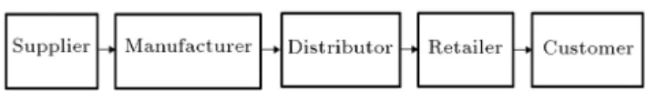
eciently with each other on the entire SCN. The concept of the SCN is presented in Figure 1 [2]. Supply Chain Management (SCM) coordinates and integrates all these activities into a smooth process. The main objective of a SCM system is to minimize system-wide costs while satisfying service-level requirements with increasing global competition, even in emergence of e-business deals. SCM is viewed as a major solution for cost reduction and protability strategies [3].
Recent studies have focused on multi-facility, multi product, and multi-period problems. Several algorithms have been developed to solve SCN problems. Many mathematical programming methods, such as Linear Programming (LP), Integer Programming (IP), and Mixed-Integer Programming (MIP), have been utilized to solve the small-scale problems. On the other
Figure 1. The concept of the supply chain network.
hand, metaheuristic algorithms, such as Genetic Algo-rithms (GA), Neural Networks (NN), and Simulated Annealing Algorithms (SAA), have been developed to solve large-scale problems, known due to the NP-hardness of a SCN. Real SCN problems have several stochastic parameters, such as demand rate and lead time. Therefore, the simulation approach can be more practical for addressing such a stochastic large-scale real world problem. Chan [4] identied seven categories of quantitative and qualitative performance measure-ment. These include cost and resource utilization as quantitative, and quality, exibility, visibility, trust, and innovativeness as qualitative.
Also, several studies proposed the simulation approach to solve the problem. The simulation ap-proach proposed by Lee et al. [5] was based on the equation of continuous portion in the SCN architecture in modelling the problem. The architecture includes and describes how these portions can be used in SCN simulation models. Joines et al. [6] utilized a SCN simulation, optimization methodology, using GA to optimize system parameters. Jang et al. [7] and Lim et al. [8] introduced a Bill Of Material (BOM) relationship between manufacturing plants. Long and Lin [9] pro-posed a framework of a multi-agent-based distributed simulation platform for SCN. Pan et al. [10] provided a systematic approach for analyzing and designing SCN construction. They utilized a simulation technique to explore the behaviour of the SCN and nd the near optimal solutions. Akgul et al. [11] commented on optimization-based methods for biofuel supply chain assessment under uncertainty. The work identies mathematical programming, as well as simulation-based methods, as being relevant to this eld. Weare and Fagerholt [12] studied optimal planning of oshore SCN. Considering major uncertainty elements, such as weather impact, on sailing and loading operations, they described how voyage-based solution methods can be used to provide decision support in the supply vessel planning process. In their proposed solution, the simulation was combined with an optimization method to create a more robust eet, and schedule solutions for supply planning. Some modelling tech-niques to model SCN under uncertainty were presented by Awudu and Zhang [13]. Their work focused on biorenery SCN, while researchers made the point that there is limited literature regarding uncertainty, specically in the biorenery SCN context. They concluded that all supply chains are under uncertainty conditions. The researchers used analytical methods and simulation-based techniques. Zengin et al. [14]
investigated discrete event simulation with its robust, accurate modelling, and analysis capabilities. Long and Zhang [15] proposed an integrated framework for agent-based inventory production-transportation modelling and distributed simulation of SCN. This extended framework provides users with a meta-agent class library and a multi-agent-based distributed platform for SCN to build an agent-based simulation model visually and rapidly using meta-agents as building blocks. Further, it supports the independent build-ing of sub-simulation models, implementbuild-ing and syn-chronizing them together in a distributed environ-ment.
Research that has utilized metaheuristic algo-rithms can be investigated as follows. Chan et al. [16] developed a hybrid GA for production-distribution problems in multi-factory SCN models, and solved a hypothetical production-distribution problem using this algorithm. Chan and Chung [17] presented an optimization algorithm to solve the problem of demand allocation, transportation, and production scheduling in a demand-driven multi-echelon distribution network, especially considering demand due date. The proposed optimization algorithm was combined with GA and the Analytic Hierarchy Process (AHP). Gen and Syarif [18] proposed a new technique, called a spanning tree-based GA, for solving production-distribution prob-lems. They integrated production, distribution, and inventory systems, so that products were produced and distributed in the right quantities, to the right customers, and at the right times. The goal was to minimize total costs while satisfying all customer demands. Syami [19] studied the traditional facility location problem considering logistic costs. To this end, two dierent heuristics, based on Lagrange re-laxation and SAA, were used. Ross [20] proposed a two-phase approach for a SCN. The rst phase includes a strategy that selects the best set of dis-tribution centers to be opened, and the second is an operational decision that includes customer and resource assignments. The SAA is applied to solve this problem. Jayaraman and Ross [21] provided a distribution network in two models, focusing on two key stages: planning and implementing. De-termining warehouse and cross-dock center allocation to open warehouses, and family product allocation from warehouse to cross-dock center are all results of solving the rst model. The second model is an operational model aiming to minimize the cost of transportation to warehouses, the cost of transporta-tion from warehouses to cross-dock centers and the cost of product distribution to the customers. SAA is used to achieve near optimal solutions for both models. Zhang et al. [22] presented an extended GA to support the multi-objective decision-making optimization for the SCN. They showed that their
proposed approach can obtain the optimal manufac-turing resource allocation plan within a reasonable time in the proposed case studies. Xian-cheng et al. [23] proposed a genetic-particle swarm optimiza-tion algorithm for closed-loop SCN. They show that their algorithm provides a new way to design closed-loop SCN and gain good convergent performance and rapidity. Furlan et al. [24], Sukumara et al. [25], and Caballero et al. [26] combined process simulation and optimization to optimize the combinatorial optimiza-tion problems.
In this research, the mathematical model from Lim et al. [8] was developed by considering capacitated warehouses and dening some new relevant variables to the basic model for each echelon to make the SCN model much more realistic. For example, in some industrial companies, such as iron melting industries, many products have particular length and width sizes, and, thus, keeping them in un-capacitated warehouses for long times is impossible. Therefore, the warehouse capacities of these companies are limited. According to Lim et al. [8] this problem is an NP-hard problem, so, two hybrid simulation-metaheuristic algorithms, called HSIM-META, were developed to solve the SCN model. The simulation is used to solve and x the routes of the SCN and computing of the total costs. Then, these feasible solutions are used as the initial population in metaheuristic algorithms to nd near optimum solutions. To the best of our knowledge, there is no similar approach in dealing with the SCN, which combines simulation and metaheuristic algorithms to solve the model. However, using simulation, or com-bining simulation with metaheuristics (OVS), is not a new approach in SCN literature, but this is the rst time that a new OVS method has been developed for the SCN. Usually, in OVS methods, the simulation replications are used to calculate the tness function. Sometimes the simulation replications are used to pro-duce a regression model to be used as the tness func-tion. Sometimes, at each iteration of the metaheuristic, whenever the algorithm wants to calculate the tness function, it replicates the simulation model to achieve this value. This novel approach connects the simulation model and the metaheuristics through construction of the initial population. Based on conjecture, wherein having an initial good feasible population, instead of random initial ones, can terminate the metaheuristics faster, the simulation model helps to produce several feasible solutions randomly in a very short time (1000 solutions in less than 1 second). This conjecture has been proved at least for the current problem, i.e. the initial high quality population can result in a faster termination. The optimum solution may be among these generated solutions, or, at least, the best solution could be a good lower bound for the main problem. This capability helps metaheuristics to start
from a good basis and to reject many non-promising solutions.
This paper is organized in the following way. In Section 2, the mathematical model is presented. In Section 3, the solution methodologies are explained by introducing GA and SAA. Then, the proposed hybrid simulation-metaheuristics (HSIM-META) are especially described with their components. The link between simulation results and metaheuristics is also presented by developing and testing three dierent scenarios. The best one has been selected based on minimizing total costs, including xed set up costs, production costs, inventory holding costs, and trans-portation costs. In Section 4, the computational results have been presented which compare the results of HSIM-META with normal GA and SAA. Finally, concluding remarks and suggestions for future research are presented in Section 5.
2. Mathematical model
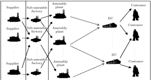
The SCN model in this study has ve echelons, in-cluding suppliers, sub assembly factories, nal assem-bly factories, DCs, and nal customers. The cost parameters assumed in the model are production, transportation, inventory holding, and facility set up costs. An example case of a SCN used for this study is presented in Figure 2.
The assumed SCN procures raw material from the suppliers and processes them into the sub-assembled products in sub-assembly factories. These sub-assembled products are then transported to the nal as-sembly factories for producing the assembled products, and, then, nal assembly products are transported to the distribution centers to fulll customer demand.
The basic formulation of the SCN problem was taken from Lim et al. [8] with some revisions, includ-ing the warehouse capacities for all factories at each echelon, and by adding some relevant variables to the basic model.
The following assumptions are made regarding the underlying SCN at each period of time:
Suppliers, manufacturing plants, DCs, customers, and products are known;
The customer demands of each product are known and condent;
The locations of the suppliers, manufacturing plants, DCs, and customers are known;
The set up time are assumed to be negligible;
All cost parameters are known and condent;
All manufacturing plants and DCs have relevant capacity for production and inventory;
Figure 2. An example of the supply chain network for this study.
The bill of material (BOM) of each sub product of any nal product is known, and the consumption ratio is 1:1.
The following notations are used: Indices
c Index of raw materials (c = 1; 2; :::; C); v Index of sub-assembled products
(v = 1; 2; :::; V );
K Index of nal assembled products (k = 1; 2; :::; K);
e Index of suppliers (e = 1; 2; :::; E); s Index of sub-assembly factories
(s = 1; 2; :::; S);
P Index of nal assembly factories (p = 1; 2; :::; P );
J Index of distribution centers (j = 1; 2; :::; J);
d Index of customers (d = 1; 2; :::; D); T Index of time periods (t = 1; 2; :::; T ). Parameters
Pcet Fixed set up cost of e for c at time
period t;
Pvst Fixed set up cost of s for v at time
period t;
Pkpt Fixed set up cost of p for k at time
period t;
Pkjt Fixed set up cost of j for k at time
period t;
Cces Unit production cost of c at e to s at
time period t;
Cvspt Unit production cost of v at s to p at
time period t;
Ckpjt Unit production cost of k at p to j at
time period t;
HCcet Unit inventory holding cost of c at e at
time period t;
HCcsvt Unit inventory holding cost of c at s to
v at time period t;
HCvst Unit inventory holding cost of v at s at
time period t;
HCvpkt Unit inventory holding cost of v at p to
k at time period t;
HCkpt Unit inventory holding cost of k at p
at time period t;
HCkjt Unit inventory holding cost of k at j at
time period t;
T Ccest Unit transporting cost of c from e to s
at time period t;
T Cvspt Unit transporting cost of v from s to p
at time period t;
T Ckpjt Unit transporting cost of k from p to j
at time period t;
T Ckjdt Unit transporting cost of k from j to d
at time period t;
Adkt Demand of k for d at time period t;
T Nce Processing time of c at e;
T Nvs Processing time of v at s;
T Nkp Processing time of k at p;
Qcet Total available production capacity of
c at e at time period t;
Qvst Total available production capacity of
v at s at time period t;
Qkpt Total available production capacity of
k at p at time period t;
Rcet Total available inventory capacity of c
at e at time period t;
Rcst Total available inventory capacity of c
Rvst Total available inventory capacity of v
at s at time period t;
Rvpt Total available inventory capacity of v
at p at time period t;
Rkpt Total available inventory capacity of k
at p at time period t;
Rkjt Total available inventory capacity of k
at j at time period t;
M A large positive integer number. Variables
Xcest Production amount of c at e to s at
the end of period t;
Xvspt Production amount of c at e to s at
the end of period t;
Xkpjt Production amount of k at p to j at
the end of period t;
Icet Inventory amount of c at e at the end
of period t;
Icsvt Inventory amount of c at s to v at the
end of period t;
Ivst Inventory amount of v at s at the end
of period t;
Ivpkt Inventory amount of v at p to k at the
end of period t;
Ikpt Inventory amount of k at p at the end
of period t;
Ikjt Inventory amount of k at j at the end
of period t;
T Rcest Transportation amount of c from e to
s at the end of period t;
T Rvspt Transportation amount of v from s to
p at the end of period t;
T Rkpjt Transportation amount of k from p to
j at the end of period t;
T Rkjdt Transportation amount of k from j to
d at the end of period t.
Wcest 8 > > < > > :
1; if transportation takes place from e to s at the end of period t
0; otherwise Wvspt 8 > > < > > :
1; if transportation takes place from s to p of v at the end of period t 0; otherwise Wkpjt 8 > > < > > :
1; if transportation takes place from p to j of k at the end of period t 0; otherwise Wkjdt 8 > > < > > :
1; if transportation takes place from j to d of k at the end of period t 0; otherwise Ucet 8 > > < > > :
1; if production takes place for c at supplier e at the end of period t 0; otherwise Uvst 8 > > > > > < > > > > > :
1; if production takes place for v at the nal assembly factory s at the end of period t
0; otherwise Ukpt 8 > > > > > < > > > > > :
1; if production takes place for k at the nal assembly factory p at the end of period t
0; otherwise Ukjt 8 > > < > > :
1; if DC j is opened for k at the end of period t 0; otherwise
The mathematical model (Problem 1) is presented as follows: Minimize X c X e X t
(PcetUcet) + (HCcetIcet)
+X
s
(CcestXcest)
+X v X s X t
(PvstUvst)
+ (HCvstIvst) +
X
p
(CvsptXvspt)
+X k X p X t
(PkptUkpt) + (HCkptIkpt)
+X
j
(CkpjtXkpjt)
+X c X s X v X t
(HCcsvtIcsvt)
+X v X p X k X t
(HCvpktIvpkt)
+X k X j X t
(PkjtUkjt) + (HCkjtIkjt)
+X c X e X s X t
(T CcestT Rcest)
+X v X s X p X t
(T CvsptT Rvspt)
+X k X p X j X t
(T CkpjtT Rkpjt)
+X k X j X d X t
(T CkjdtT Rkjdt) (1)
St: X
s
(T NceXcest) QcetUcet; 8c; e; t; (2)
X
p
(T NvsXvspt) QvstUvst; 8v; s; t; (3)
X
j
(T NkpXkpjt) QkptUkpt; 8k; p; t; (4)
Icet RcetUcet; 8c; e; t; (5)
Icsvt RcstUvst; 8c; s; v; t; (6)
Ivst RvstUvst; 8v; s; t; (7)
Ivpkt RvptUkpt; 8v; p; k; t; (8)
Ikpt RkptUkpt; 8k; p; t; (9)
Ikjt RkjtUkjt; 8k; j; t; (10)
Xcest MUcet; 8c; e; s; t; (11)
Xvspt MUvst; 8c; e; s; t; (12)
Xkpjt MUkpt; 8c; e; s; t; (13)
T Rcest MWcest; 8c; e; s; t; (14)
T Rvspt MWvspt; 8v; s; p; t; (15)
T Rkpjt MWkpjt; 8k; p; j; t; (16)
T Rkjdt MWkjdt; 8k; j; d; t; (17)
X
s
Xcest+ Icet
X
s
T Rcest Icet 1= 0; 8c; e; t;
(18) X
p
Xvspt+ Ivst
X
p
T Rvspt Ivst 1= 0; 8v; s; t;
(19) X
j
Xkpjt+ Ikpt
X
j
T Rkpjt Ikpt 1= 0; 8k; p; t;
(20) Ikjt 1 Ikjt T Rkjdt+ Adkt= 0; 8k; j; d; t; (21)
X p Xvspt X c X e Xcest X c
Icsvt 1; 8v; s; t;
(22) X j Xkpjt X v X s Xvspt X v
Ivpkt 1; 8k; p; t;
(23) Xcest; Xvspt; Xkpjt 0 8c; e; s; v; p; k; j; t; (24)
Icmt; Icsvt; Ivst; Ivpkt; Ikpt; Ikjt 0
8c; m; s; v; p; k; j; t; (25) T Rcmst; T Rvspt; T Rkpjt; T Rkjdt 0
8c; m; s; v; p; k; j; d; t; (26) Ucet;Uvst;Ukpt;Ukjt;Wcest;Wvspt; Wkpjt;Wkjdt2 f0; 1g
(27) The objective function of this model is to minimize the total costs, including set up, production, inven-tory holding, and transportation costs through the model. Constraints (2)-(4) represent the capacity restrictions for each supplier, sub-assembly factory, and nal assembly factory. Constraints (5)-(10) represent the capacity restriction for the supplier, warehouse, sub-assembly warehouse, nal assembly warehouse, and DC. Constraints (11)-(13) ensure that a set up event occurs when a factory manufactures an item such as raw material, sub-assembled product, or nal-assembled product. Constraints (14)-(17) imply that a link among plants exists if the transportation quantities are non-zero. Constraints (18)-(21) represent a balance equation that denes the inventory levels for items c, v, and k at the end of period t at each plant, and DC results from production and transportation procedures. Constraints (22) and (23) ensure that the external demands must be satised. Constraints (24)-(26) represent the non-negativity restrictions on the decision variables. Constraint (27) shows the integer 0-1 variables. It should be mentioned that Constraint sets (5)-(10) have been added to the basic model of Lim et al. [8] as limited capacity warehouses of factories at each echelon.
3. Solution methodologies
At rst, general metaheuristic algorithms, including the Genetic Algorithm (GA) and the Simulated An-nealing Algorithm (SAA) are briey described, and, then, the proposed HSIM-GA and HSIM-SAA and their components are especially described.
3.1. Genetic algorithm in general
The Genetic Algorithm (GA) is a well-known meta-heuristic optimization technique originally developed
by Holland [27]. Vose [28] provided the whole concept of the basic GA. R.L. Haupt and S.E. Haupt [29] under-took a brief study, including some of the latest research results on applying GA. Briey, the GA mechanism is based on a natural selection process that starts with an initial set of random solutions (population). Each individual in the population (chromosome) indicates a solution to the problem. During a generation, the chromosomes are evaluated using a cost function. In order to produce the next generation, two operators are used in GA. The rst, called the crossover, merges two chromosomes of a current generation to create ospring, and the other, called, mutation, modies a chromosome. Then, based on cost function values, some parents and ospring having better values of cost function, form a new generation. In this way, better chromosomes of successive generations have higher probabilities of being selected and the algorithm converges to the best chromosome that expectantly indicates the optimum or near optimal solution to the problem after several generations. In general, GA can nd the global optimum solution with a high probability.
3.2. Simulated annealing algorithm in general SAA is a randomized local search method based on simulation of metal annealing. The procedure was popularized by Krikpatrik et al. [30] and is based on the work carried out by Metropolis et al. [31] (also called the Metropolis algorithm) in statistical mechanics. SAA emulates the physical process of annealing, which attempts to force a system to its lowest energy state through a controlled cooling procedure. In a physical system with a large number of atoms, equilibrium may be characterized as the minimal value for the energy of the system. This is accomplished by a slow cooling of the temperature. Then, the system is said to be at thermal equilibrium at temperature T if the probability of being in state i with energy Ei follows the Bultzen
distribution:
P robfx = ig = exp n
Ei
KBT
o P
expf Ei
KBTg
; (28)
where KBis the Bultzen constant and the sum extends
to all possible states. By moving the atoms randomly to new congurations, dierent energy changes are induced (E). If the increment is negative, the new conguration is accepted as a new state, but if the conguration has higher energy than the previous state, it is only accepted with a certain probability, as follows:
exp
E KBT
: (29)
By repeating these steps, it is shown that the accepted congurations converge to the Bultzen distribution
after some indeterminate number of iterations at each particular temperature. The procedure may be easily applied to a large number of optimization problems, where the objective function plays the role of energy. In this context, the temperature is a control parameter to dene large or small moves for the optimization variables.
3.3. Proposed hybrid
simulation-metaheuristics algorithm (HSIM-META)
As mentioned earlier, Problem 1 is an NP-hard problem and, so, metaheuristic algorithms can be potentially appropriate for solving the problem. On the other hand, the SCN has several stochastic parameters which cannot be dealt with via mathematical programming approaches, especially in large scale problems. There-fore, the simulation is used to model the real world SCN problems. First, a mathematical model is constructed similar to Problem 1 and, then, this model is used to construct the corresponding simulation model. All constraints in Problem 1 are coded in the simulation software in such a way that each run results in a feasible solution. Then, the simulation model is run and the best production-distribution routes for each customer are obtained. Also, each run is terminated when all demands of customers are satised. Next, the output solutions of simulation are used as the initial population in the proposed tuned metaheuristics. The metaheuristics run and its circle is repeated until the stopping criteria are satised. Therefore, the simulation model has two key specications in the tuned parameter proposed HSIM-META algorithm. First, it produces some feasible solutions which can be used in the GA and SAA as initial population, and, second, it covers and handles the stochastic behaviour of the SCN. In the next subsection, we describe the essential components of the HSIM-GA and HSIM-SAA in detail.
3.3.1. The chromosome representation of HSIM-GA The rst important step in utilizing the proposed HSIM-GA algorithm is the chromosome representation. We design a heuristic chromosome, which can generate feasible solutions and which satises the majority of constraints (Constraint sets (2)-(17)). Our chromo-some structure is a NT super matrix, where, N is the
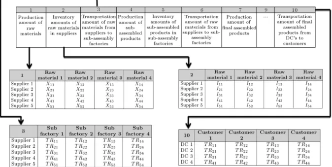
number of the submatrix, which illustrates suppliers, sub-assembly factories, nal assembly factories, DCs and customers, and T is the period of time. An example of the chromosome structure is shown in Figure 3. In this gure, we describe submatrix numbers 1, 2, 3, and 10 as an example.
The main important questions related to the pro-duction, warehousing, and transportation capacities of the SCN at each echelon are as follows:
Figure 3. An example of the chromosome structure.
I. How many products should be produced at each factory?
II. How many products should be transported to the next echelon?
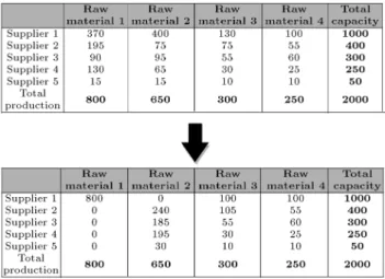
To answer these questions, we introduce a heuris-tic method for randomly generating a feasible initial population which can consider these constraints. The following example presents the proposed heuristic:
X1+ X2+ X3+ X4+ X5= 2000; (30)
X1 1100; (31)
X2 500; (32)
X3 400; (33)
X4 300; (34)
X5 100: (35)
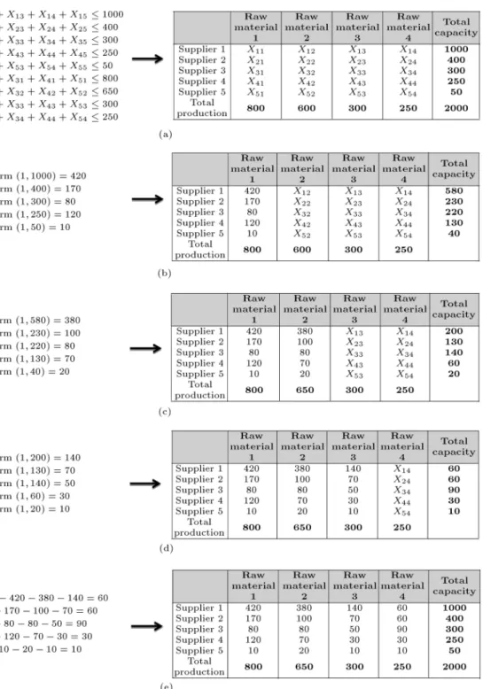
Suppose that the above model represents the rst row of submatrix 1, including the production amount of raw material, type 1, at the suppliers. Constraint (30) shows that the total amount of raw material produced by the suppliers is equal to 2000. Also, Constraint sets (31)-(35) implies that the maximum production capacity of suppliers 1, 2, 3, 4 and 5 to produce raw material type 1 are 1100, 500, 400, 300 and 100, respectively. According to the above information, we can infer that suppliers 2, 3, 4, and 5 can produce, totally, 1300 units of raw material type 1 if they work with maximum capacity. Also, we can conclude that
supplier 1 should, at least, produce 700 units of raw material, type 1, to satisfy Constraint (30). Therefore, if suppliers 3, 4, and 5 work with maximum capacity, they can produce 800 units of raw material type 1, totally, and supplier 2 should at least produce 200 units of raw material, type 1. Also, suppliers 4 and 5 can produce totally 400 units of raw material, type 1, if they work at maximum capacity. Therefore, supplier 3 should at least produce 200 units of raw material, type 1, to satisfy Constraint (30). Next, we can conclude that supplier 4 should at least produce 200 units of raw material, type 1, to satisfy Constraint (30). According to the information, we could ll submatrix 1 as follows: X1= Uniform (700; 1100) = 1000; (36)
X2 500; (37)
X3 400; (38)
X4 300; (39)
X5 100; (40)
X2+ X3+ X4+ X5= 1000; (41)
X2= Uniform (200; 500) = 400; (42)
X3+ X4+ X5= 600; (43)
X3= Uniform (200; 400) = 300; (44)
X4= Uniform (200; 300) = 250; (46)
X5= 2000 1000 400 300 250 = 50: (47)
A graphical representation of the described heuristic method can be found in Figure 4(a)-(e), in which all manufacturing plants, such as suppliers, sub-assembly factories, and nal assembly factories, produce accord-ing to the their production capacity constraints (this procedure is utilized for Constraint sets (2)-(17).
3.3.2. Initialization of HSIM-GA
The input parameters of our HSIM-GA is the popu-lation size (NP op), which shows the total number of
chromosomes in each generation, crossover probability (Pc) and mutation probability (Pm).
3.3.3. The cross over operator of HSIM-GA
The goal of cross over is to explore new solution space. The cross over operator corresponds to exchanging the parts of the strings of selected parents. In general, there
are three ways to keep the initial solutions feasible by cross over, as follows:
Assume penalty functions for infeasible solutions;
Return the infeasible solutions to feasible solutions by special techniques;
Keep every new generated solution feasible.
After generating feasible submatrixes as parents, the proposed cross over operator is used as follows:
1. Two chromosomes are selected according to the roulette wheel selection method;
2. Every cell of parent 1 is added to the corresponding cell of parent 2, then, this value is divided by two. In other words, the average of the two parents is called the ospring. These calculations are repeated for all submatrixes at each period of time.
This cross over operator ensures that all generated osprings are feasible and one never comes out of the feasible region. An example of the proposed cross over operator of submatrix 1 is illustrated in Figure 5. 3.3.4. The mutation operator of HSIM-GA
Mutation is undertaken to prevent premature conver-gence and to explore new solution space. We introduce a new mutation operator that keeps each generated so-lution feasible. We consider submatrix 1 to present our mutation operator of HSIM-GA. First, we randomly select a supplier and allocate total productions to it, as follows: One cell of the submatrix is selected and total production is assigned to it. Next, the other submatrix cells are updated considering the total production and capacity of factory constraints. An example of the mutation operator is shown in Figure 6.
At the second step, the essential components of the HSIM-SAA are presented as follows.
Figure 6. An example of the mutation operator.
3.3.5. Initialization of HSIM-SAA
The input parameters of the SAA are: Initial tempera-ture (T0), which is the starting temperature point and
the temperature decreasing rate ().
3.3.6. Solution representation of HSIM-SAA
The solution representation in the HSIM-SAA is similar to the ones described in \The chromosome representa-tion" for HSIM-GA.
3.3.7. Neighborhood representation of HSIM-SAA To present the neighborhood structure, the proposed mutation operator of HSIM-GA, described in \The mutation operator" is utilized to avoid fast convergence of the HSIM-SAA.
3.3.8. Initial temperature
A suitable initial temperature is one that results in an average increase of acceptance probability near to one. The value of initial temperature will clearly depend on the scaling of tness and, hence, it should be problem-specied. Therefore, we rst generate a large set of
random solutions, then, a standard division of them is calculated and used to determine the initial tempera-ture in such a way that the acceptance probability of primary generations reached 0.95. Consequently, the initial T is set to 1500, based on some preliminary parameter selection examinations, which are described in Subsection 4.1.
3.3.9. Stopping criteria
In general, the algorithms could be stopped in the following ways:
After a predened number of generations;
When an individual solution reaches a predened level of tness;
When the variation of individuals from one genera-tion to the next generagenera-tion reaches a predened level of stability.
In this paper, the algorithms will be stopped according to the rst way, in which, if there is no improvement in the best tness value for the 50 genera-tions, the algorithms will stop. This stopping criterion is used for both HSIM-GA and HSIM-SAA algorithms. Figures 7 and 8 depict the owchart of the proposed Hybrid Simulation-Genetic Algorithm (HSIM-GA) and a Hybrid Simulation-Simulated Annealing Algorithm (HSIM-SAA), respectively.
3.3.10. Allowing infeasibility
To simplify the escape process from local optimum so-lutions, the chromosome is allowed to be infeasible, but is penalized according to the amount of infeasibility. An ecient penalty formulation, which is dynamic, is applied in such a way that explores the space in the rst and results in infeasible solutions at the end of the evolution. A general form of a distance based penalty method, incorporating a dynamic aspect, is based on the length of the search area for our minimization problem:
Fp(x; t) = f(x) + s
X
s=1
pst; (48)
where ps is a relative scaling for violation of
chro-mosomes from constraint s, and t is the generation number. This penalty formulation is capable of visiting highly infeasible solutions at the rst steps of the search. By gradually increasing the penalty amount imposed on bad moves, the next solutions tend to be close to the feasible region (this procedure is used for Constraint sets (18)-(23).
4. Computational results
All computations were carried out on a PC using a Core i5 with 2.4 GHz CPU, and 4 GB of RAM.
Figure 7. The owchart of the proposed HSIM-GA.
Enterprise Dynamics (ED) 8.2 [32] was used as the simulation software and all constraints in problem 1 were coded in ED 8.2. MATLAB V7.13.0.564, R2011b was used to code the metaheuristics, and the linear programming models have been solved using CPLEX 9.0. Also, Minitab 16 software has been used to tune the parameters. According to Lim et al. [8], the backlogging is not planned in the model and unsatised demand in the previous periods is not transferred to the next. The order quantity is computed according to the BOM ratio, which is set to 1 in this study for each echelon. We design a simulation model to impose any excessive costs onto the model, in such a way that when the demand of the last nal customer is satised, all manufacturing plants at each echelon are stopped. We link the simulation model to the Microsoft Excel so that after each simulation run, the simulation results are exported to the Excel sheets, and the total xed and variable costs are calculated. Then, the simulation model is replicated and the best
production-Figure 8. The owchart of the proposed HSIM-SAA.
distribution routes for each customer are obtained. After closing non-economic facilities and warehouses in the simulation model, it is replicated again and total costs are computed. To use the results of the simulation model, each problem is replicated 500 times and the results are saved in Microsoft Excel sheets. Regardless of the volume of goods transported among the dierent echelons, the simulation model can help to determine the best distribution routes in the SCN. In the second phase, these production-distribution routes are xed in the simulation model, and, again, the model is replicated 100 times to determine the near optimum volumes (transportation volumes among ech-elons). Therefore, after 100 replications, 100 feasible solutions are saved in the Microsoft Excel sheets. For each feasible solution, the average total costs are
calculated in two ways; by xing the routes (by closing the non-economic factories and warehouses according to the previous results) and without xing routes. In this paper, we use the second way because it produces lower costs.
Ten dierent test problems were created; the size of each test problem is shown in Table 1. All test problems have 4 nal products. The total costs include transportation, production, inventory holding and xed set up costs from supplier to nal customer at each echelon. All test problems are generated using uniform distributions, which are depicted in Tables 2 to 5, respectively. Every factory produces four types of product, including four raw materials in the suppliers, four sub-assembled products in the sub-assembly fac-tories, and four nal assembled products in the nal assembly factories at each echelon. The processing time of raw materials in the suppliers and the sub products in the sub-assembly factories follow a uniform distribution U(10; 15). The processing time of nal products in nal assembly factories follows a uniform distribution U(15; 20). The customer demand of each product is an integer number uniformly distributed from U(30; 60). Also, the maximum storage capacity of raw materials in the supplier warehouse, the sub products in the sub-assembly factory warehouse, the nal product in the nal assembly factory warehouse, and the nal product in DCs are equal at 70, 70, 75, and 75, respectively.
4.1. Tuning the parameters
The initial parameters of our HSIM-GA include cross over (Pc) and mutation (Pm), and the initial parameter
of our HSIM-SAA is initial temperature (T0), which is
the starting temperature point, and the temperature decreasing rate (). We used the Taguchi method in designing the experiments (DOE) [33]. In the Taguchi method, the results are transferred into a measure called a signal to noise (S=N) ratio. The formulation of this ratio is dierent for each objective (maximization or minimization). Eq. (49) represents the (S=N) ratio for minimization objectives:
S=N = 10 log 1=nXn
i=1
y2 i
!
; (49)
in which, n and yi indicate the number of replications
and process response values at the i'th replication. In the DOE, we chose the orthogonal array of L9both for
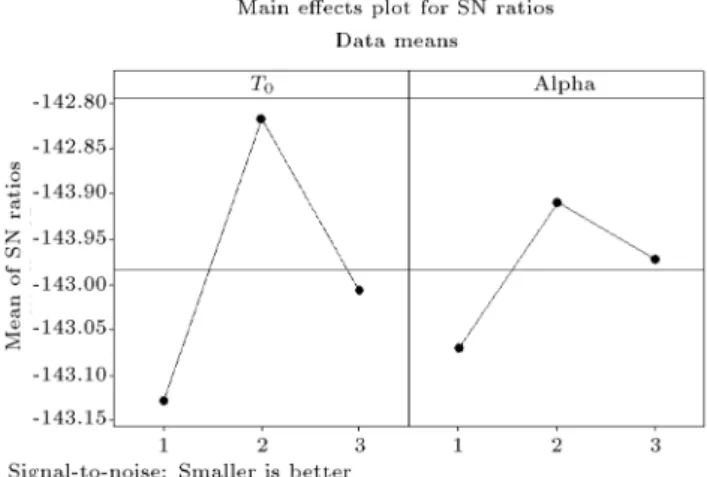
HSIM-GA and the HSIM-SAA. The initial parameter values, after the sensitivity analysis of the factors, are shown in Tables 6 and 7. Figures 9 and 10 depict the averaged S=N ratio for each factor level. Also, the optimum combinations of the parameters for each META, which include GA and HSIM-SAA, are shown in Table 8.
Table 1. The size of test problems. Problem
sizes
Number of suppliers
Number of sub-assembly factory
Number of nal assembly factory
Number of DCs
Number of customer
1 1 2 2 1 2
2 2 1 2 2 2
3 2 2 1 2 3
4 2 2 2 2 3
5 3 2 3 2 3
6 3 3 2 3 3
7 4 3 5 4 3
8 4 3 4 4 4
9 5 4 4 4 4
10 5 5 5 4 4
Table 2. Transportation costs among echelons. Transporter cost
from supplier to sub-assembly factory
Transporter cost from sub-assembly
factory to nal assemble factory
Transporter cost from nal assembly
factory to DC
Transporter cost from DC to nal customer Transporter costs U (200, 700) U (400, 800) U (200, 600) U (200, 700)
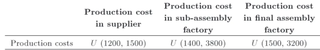
Table 3. Production costs of manufacturing plants at each echelon. Production cost
in supplier
Production cost in sub-assembly
factory
Production cost in nal assembly
factory Production costs U (1200, 1500) U (1400, 3800) U (1500, 3200) Table 4. Inventory holding costs of manufacturing plants and warehouses at each echelon.
Inventory holding cost in supplier
Inventory holding cost in sub-assembly factory
Inventory holding cost in nal assembly factory
Inventory holding cost
in DC Inventory holding costs U (50, 80) U (40, 100) U (50, 80) U (60, 90)
Table 5. Fixed set up costs of manufacturing plants and warehouses at each echelon. Supplier Sub-assembly factory Final assembly factory DC Fixed set up
costs U (1200000, 1600000) U (2000000, 4000000) U (5000000, 9000000) U (500000, 800000)
4.2. Analysis of results
In order to use HSIM-META to obtain near optimum solutions, three dierent scenarios were developed to link the output data of the simulation model in the tuned-parameter, HSIM-META. The scenarios, as fol-lows, determine how the randomly generated solutions in the simulation model must be used as the initial population in HSIM-META:
- Scenario 1: 10 best simulation solutions (regarding their objective function) are used;
- Scenario 2: 10 best simulation solutions, together with 10 medium solutions, are use;
- Scenario 3: 10 best simulation solutions, 10 medium solutions, and 10 worst solutions are used.
After several experiments using MATLAB soft-ware, it was shown that Scenario 1 is the best. Then, we link the output of the rst 10 best simulation solutions in tuned-parameter HSIM-META.
To test the performance of HSIM-META, we com-pared META, including GA and
HSIM-Table 6. The initial parameter ranges in HSIM-GA. Parameters Factor levels
1 2 3
Npop 300 500 700
Pc 0.85 0.9 0.95
Pm 0.01 0.02 0.03
Table 7. The initial parameter ranges in HSIM-SAA. Parameters Factor levels
1 2 3
T0 1000 1500 2000
0.9 0.95 0.99
Figure 9. Factor level of the proposed HSIM-GA.
Figure 10. Factor level of the proposed HSIM-SAA.
SAA, with general GA and SAA, without using the simulation result as the initial population for the test problems. Also, we utilized the Average Relative Per-centage Deviation (ARPD) to compare the algorithms, according to the following formulas:
RPDj = Zs(j) minmin s(j)
s(j) 100 j = 1; :::; n; (50)
Table 8. The optimum parameter levels. Hybrid
metaheuristics Parameters
Optimum amounts
HSIM-GAA
Npop 500
Pm 0.02
Pc 0.9
Pr= 1 (Pc+ Pm) 0.08
HSIM-SAA T0 1500
0.95
Figure 11. The Tukey's Honestly Signicant Dierence (HSD) for the small sized problems.
ARPD = Pn
i=1RPD
n ; (51)
where, Zs is the objective function value for a given
algorithm, mins is the best value of the objective
function between both algorithms, and n is the row number of small size or large size problems.
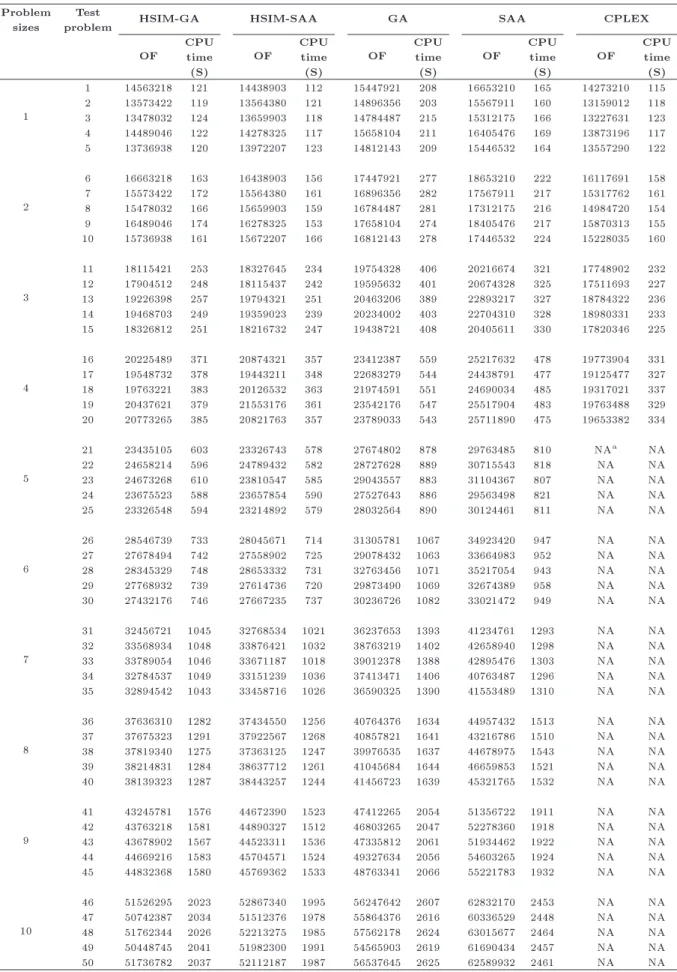
The results of the proposed GA, HSIM-SAA, GA, and SAA are presented in Table 9. We designed 50 cases for the test problems. Each problem size was replicated ve times and the optimum solu-tions of the objective function and the CPU time were recorded. To investigate the solution quality of the proposed algorithms, the optimum solution of each test problem is obtained by CPLEX. The last two columns of Table 9 report the objective function and CPU time for the CPLEX. We limited the computational time of CPLEX to 2000 seconds. Not obtaining the global optimum solution within this time limitation is meant as \Not available (Out of CPU time)".
In order to statistically compare algorithm qual-ity, Tukey's Honestly Signicant Dierence (HSD) test is applied. Using this test, we are able to reveal signicant dierences between algorithms. As shown in Figure 11, the dierences are not very meaningful among HSIM-GA, HSIM-SAA, GA, SAA and CPLEX for the small-sized problems. Thus, it can be concluded that two meta-heuristics, along with the others, are able to nd good solutions.
Figures 12 and 13 show the Average RPD (ARPD) of the objective function and the CPU time
Table 9. The computational results for Objective Function (OF) and CPU time.
Problem
sizes problemTest HSIM-GA HSIM-SAA GA SAA CPLEX
OF CPUtime (S)
OF CPUtime (S)
OF CPUtime (S)
OF CPUtime (S)
OF CPUtime (S) 1
1 14563218 121 14438903 112 15447921 208 16653210 165 14273210 115 2 13573422 119 13564380 121 14896356 203 15567911 160 13159012 118 3 13478032 124 13659903 118 14784487 215 15312175 166 13227631 123 4 14489046 122 14278325 117 15658104 211 16405476 169 13873196 117 5 13736938 120 13972207 123 14812143 209 15446532 164 13557290 122
2
6 16663218 163 16438903 156 17447921 277 18653210 222 16117691 158 7 15573422 172 15564380 161 16896356 282 17567911 217 15317762 161 8 15478032 166 15659903 159 16784487 281 17312175 216 14984720 154 9 16489046 174 16278325 153 17658104 274 18405476 217 15870313 155 10 15736938 161 15672207 166 16812143 278 17446532 224 15228035 160
3
11 18115421 253 18327645 234 19754328 406 20216674 321 17748902 232 12 17904512 248 18115437 242 19595632 401 20674328 325 17511693 227 13 19226398 257 19794321 251 20463206 389 22893217 327 18784322 236 14 19468703 249 19359023 239 20234002 403 22704310 328 18980331 233 15 18326812 251 18216732 247 19438721 408 20405611 330 17820346 225
4
16 20225489 371 20874321 357 23412387 559 25217632 478 19773904 331 17 19548732 378 19443211 348 22683279 544 24438791 477 19125477 327 18 19763221 383 20126532 363 21974591 551 24690034 485 19317021 337 19 20437621 379 21553176 361 23542176 547 25517904 483 19763488 329 20 20773265 385 20821763 357 23789033 543 25711890 475 19653382 334
5
21 23435105 603 23326743 578 27674802 878 29763485 810 NAa NA
22 24658214 596 24789432 582 28727628 889 30715543 818 NA NA
23 24673268 610 23810547 585 29043557 883 31104367 807 NA NA
24 23675523 588 23657854 590 27527643 886 29563498 821 NA NA
25 23326548 594 23214892 579 28032564 890 30124461 811 NA NA
6
26 28546739 733 28045671 714 31305781 1067 34923420 947 NA NA
27 27678494 742 27558902 725 29078432 1063 33664983 952 NA NA
28 28345329 748 28653332 731 32763456 1071 35217054 943 NA NA
29 27768932 739 27614736 720 29873490 1069 32674389 958 NA NA
30 27432176 746 27667235 737 30236726 1082 33021472 949 NA NA
7
31 32456721 1045 32768534 1021 36237653 1393 41234761 1293 NA NA 32 33568934 1048 33876421 1032 38763219 1402 42658940 1298 NA NA 33 33789054 1046 33671187 1018 39012378 1388 42895476 1303 NA NA 34 32784537 1049 33151239 1036 37413471 1406 40763487 1296 NA NA 35 32894542 1043 33458716 1026 36590325 1390 41553489 1310 NA NA
8
36 37636310 1282 37434550 1256 40764376 1634 44957432 1513 NA NA 37 37675323 1291 37922567 1268 40857821 1641 43216786 1510 NA NA 38 37819340 1275 37363125 1247 39976535 1637 44678975 1543 NA NA 39 38214831 1284 38637712 1261 41045684 1644 46659853 1521 NA NA 40 38139323 1287 38443257 1244 41456723 1639 45321765 1532 NA NA
9
41 43245781 1576 44672390 1523 47412265 2054 51356722 1911 NA NA 42 43763218 1581 44890327 1512 46803265 2047 52278360 1918 NA NA 43 43678902 1567 44523311 1536 47335812 2061 51934462 1922 NA NA 44 44669216 1583 45704571 1524 49327634 2056 54603265 1924 NA NA 45 44832368 1580 45769362 1533 48763341 2066 55221783 1932 NA NA
10
46 51526295 2023 52867340 1995 56247642 2607 62832170 2453 NA NA 47 50742387 2034 51512376 1978 55864376 2616 60336529 2448 NA NA 48 51762344 2026 52213275 1985 57562178 2624 63015677 2464 NA NA 49 50448745 2041 51982300 1991 54565903 2619 61690434 2457 NA NA 50 51736782 2037 52112187 1987 56537645 2625 62589932 2461 NA NA aNA: Not Available (out of CPU time).
Figure 12. The ARPD for objective function of the algorithms.
Figure 13. The ARPD for computational time of the algorithms.
of the proposed algorithms. According to the ARPD factor, HSIM-GA has better quality, with 0.54, 10.29, and 19.84 deviations, against HSIM-SAA, GA and SAA, respectively. In terms of the CPU time index, the HSIM-SAA obtained better CPU time, with 3.33, 50.75 and 31.68 deviations, against HSIM-GA, GA and SAA, respectively. Also, Figures 14 and 15 show the 95% condence intervals of RPD for the objective function and CPU time indices, respectively. To sum up, we can see that HSIM-GA gives better results than all other algorithms in terms of the objective function, and the HSIM-SAA has better results regarding the CPU time index for all problem sizes.
5. Conclusion and suggestions for future work In this paper, a new model and two hybrid algorithms were developed to address the so-called SCN problem. The algorithms combined a simulation technique with two metaheuristic algorithms (GA and SAA), called HSIM-META, to solve such an NP-hard problem,
Figure 14. 95% condence intervals of RPD of objective function.
Figure 15. 95% condence intervals of RPD of CPU time.
which is the main contribution of the current research. First, the mathematical programming model of the SCN was developed, assuming limited capacities for the model warehouses, and then the corresponding simula-tion model was built. The simulasimula-tion model was used to determine the best production-distribution routes and to close non-economic facilities and warehouses in the SCN model. After xing the routes, several random feasible solutions were generated by the simulation model using 3 dierent scenarios and by selecting the best one. Then, 10 best feasible solutions were selected as the initial population for HSIM-META. This version of OVS is a novel approach in OVS literature. It benets from the ability of the simulation technique to produce several random feasible solutions and also from the optimization engine of metaheuristics. To test the performance of our HSIM-META algorithm, 50 numerical test problems were developed and solved using the algorithms. As the results show, combining simulation with the metaheuristic algorithms has the advantages of both methods and can escape from the local optimal solution and nd near optimal solutions. Analysis of the results shows that the HSIM-META containing HSIM-GA and HSIM-SAA has better qual-ity of solutions, regarding the objective function and
CPU time, than general GA and SAA. According to the ARPD comparisons, HSIM-GAA has better quality solutions than GA, SAA, and HSIM-SAA in terms of the objective function, and the HSIM-SAA is faster in comparison to GA, SAA, and HSIM-GA. For future research, other metaheuristic algorithms can be considered and linked to the simulation technique. Also, shortage costs can be investigated in the SCN to develop a new mathematical model. To expand the current model, our suggestion is to consider the pricing factor in the model, i.e. consider some active competi-tors in the market, whose sales volume and prices can aect product prices and demands, which could make the model much more realistic. In this new concept, which integrates SCN with market planning, an agent-based simulation modelling is highly recommended.
References
1. Thomas, D.J. and Grin, P.M. \Coordinated supply chain management", Eur. J. of Oper. Res., 94(1), pp. 1-15 (1996).
2. Pasandide, S.H.R., Niaki, S.T.A. and RoozbehNia, A. \An investigation of vendor-managed inventory application in supply chain: The EOQ model with shortage", Int. J. of Adv. Manuf. Technol., 49, pp. 329-339 (2010).
3. Tyana, J. and Wee, H.M. \Vendor managed inventory: A survey of the Taiwanese grocery industry", J. Purch. Supply Manage., 9, pp. 11-18 (2003).
4. Chan, F.T.S. \Performance measurement in a supply chain", Int. J. of Adv. Manuf. Technol., 21, pp. 534-548 (2003).
5. Lee, Y.H., Cho, M.K., Kim, S.J. and Kim, Y.B. \Supply chain simulation with discrete-continuous combined modelling", Comput. & Ind. Eng., 43, pp. 375-392 (2002).
6. Joines, J.A., Kupta, D., Gokce, M., King, R.E. and Kay, M.G. \Supply chain multi objective simulation optimization", In: Proceeding of the 2002 Winter Simulation Conference, pp. 1306-1314 (2002).
7. Jang, Y.J., Jang, S.Y., Chang, B.M. and Park, J.W. \A combined model of network design and pro-duction/distribution planning for a supply network", Comput. & Ind. Eng., 43, pp. 263-281 (2002).
8. Lim, S.J., Jeong, S.J., Kim, K.S. and Park, M.W. \A simulation approach for production-distribution planning with consideration given to replenishment policies", Int. J. of Adv. Manuf. Technol., 27, pp. 593-603 (2006).
9. Long, Q.Q. and Lin, J. \Architecture of multi-agent based distributed simulation platform for supply chain", Comput. Integer. Manuf. Syst., 16(4), pp. 817-827 (2010).
10. Pan, N.H., Lee, M.L. and Chen, S.Q. \Construction material supply chain process analysis and
optimiza-tion", J. of Civil. Eng. & Manage., 17(3), pp. 357-370 (2011).
11. Akgul, O.A., Zamboni, F., Bezzo, N.S. and Papa-georgiou, L.G. \Optimization-based approaches for bioethanol supply chains", Ind. & Eng. Chem. Res., 50(9), pp. 4927-4938 (2011).
12. Weare, E. and Fagerholt, K. \Robust supply vessel planning", Proceedings of 5th International Confer-ence, INOC 2011, Hamburg, Germany, pp. 559-573 (2011).
13. Awudu, I. and Zhang, J. \Uncertainties and sustain-ability concepts in biofuelsupply chain management: A review", Renewable and Sustainable Energy Reviews., 16(2), pp. 1359-1368 (2012).
14. Zengin, A., Sarjoughian, H. and Ekiz, H. \Discrete event modelling of swarm intelligence based routing in network systems", Inform Sciences, 222(10), pp. 81-98 (2013).
15. Long, Q. and Zhang, W. \An integrated framework for agent based inventory-production-transportation mod-elling and distributed simulation of supply chains", Inform Sciences, 277, pp. 567-581 (2014).
16. Chan, F.T.S., Chung, S.H. and Wadhwa, S. \A hybrid genetic algorithm for production and distribution", Omega, 33(4), pp. 345-355 (2005).
17. Chan, F.T.S. and Chung, S.H. \Multi-criterion genetic optimization for due date assigned distribution net-work problems", Decis. Support Syst., 39(4), pp. 661-675 (2005).
18. Gen, M. and Syarif, A. \Hybrid genetic algorithm for multi-time period production-distribution planning", Comput. & Ind. Eng., 48(4), pp. 779-809 (2005).
19. Syami, S.S. \A model and methodologies for the loca-tion problem with logistical components", Comput. & Oper. Res., 29, pp. 1173-1193 (2002).
20. Ross, A.D. \A two-phased approach to the supply network reconguration problem", Eur. J. of Oper. Res., 122, pp. 18-30 (2002).
21. Jayaraman, V. and Ross, A.D. \A simulated anneal-ing methodology to distribution network design and management", Eur. J. of Oper. Res., 144, pp. 629-645 (2002).
22. Zhang, W.Y., Zhang, S., Cai, M. and Huang, J.X. \A new manufacturing resource allocation method for supply chain optimization using extended genetic algorithm", Int. J. of Adv. Manuf. Technol., 53, pp. 1247-1260 (2011).
23. Xian-cheng, Z., Zhi-xue, Z., Kai-jun, Z. and Cai-hong, H. \Remanufacturing closed-loop supply chain network design based on genetic particle swarm opti-mization algorithm", J. Cent. South University, 19, pp. 482-487 (2012).
24. Furlan, F.F., Costa, C.B., Cruz, A.J., Secchi, A.R., Soares, P. and Giordano, R.C. \Integrated tool for simulation and optimization of a rst and second
generation ethanol-from-sugarcane production plant", Comput. Aided. Chem. Eng., Elsevier., 30, pp. 81-85 (2012).
25. Sukumara, S.J., Amundson, W., Faulkner, F., Badur-deen and Seay, J. \Multidisciplinary approach in devel-oping region specic optimization tool for sustainable bio rening", Comput. Aided. Chem. Eng., Elsevier, 30, pp. 157-161 (2012).
26. Caballero, J.A., Navarro, M.A. and Grossmann, I.E. \Hybrid simulation-optimization logic based algo-rithms for the rigorous design of chemical process", Comput. Aided Chem. Eng., Elsevier, 30, pp. 582-586 (2012).
27. Holland, J.H. Adaption in Natural and Articial Sys-tems: An Introductory Analysis with Applications to Biology, Control and Articial Intelligence, Michigan: University of Michigan Press (1975).
28. Vose, M.D. \Generalizing the notion of schema in genetic algorithms", Articial Intelligence, 50, pp. 385-396 (1991).
29. Haupt, R.L. and Haupt, S.E., Practical Genetic Algo-rithms, New York: Wiley (2004).
30. Kirkpatrick, S., Gelatt, C.D. and Vecchi, M.P. \Op-timization by simulated annealing", Science, 220, pp. 671-679 (1983).
31. Metropolis, N., Rosenbluth, A., Rosenbluth, M., Teller, A. and Teller, E. \Equations of state calcula-tions by fast computing machines", J. of Chem. Phys., 21, pp. 1087-1092 (1953).
32. Enterprise Dynamic, 8.2, www.incontrolsim.com. Am-sterdam, Netherland.
33. Montgomery, D.C., Design and Analysis of Experi-ments, Arizona, John Wiley and Sons (2005).
Biographies
Ramtin Rooeinfar received BS and MS degrees in Industrial Engineering from Islamic Azad University, Qazvin, Iran, in 2009 and 2012, respectively. He is currently a PhD degree candidate of Industrial Engi-neering at Islamic Azad University, South Tehran, Iran. His research interests are mathematical programming, metaheuristic algorithms, systems simulation, supply chain management, and facility location problems. He is currently working on exible ow shop scheduling problems and bi-objective methods.
Parham Azimi was born in 1974. He received BS, MS and PhD degrees in Industrial Engineering from Sharif University of Technology, Tehran, Iran, in 1996, 1998 and 2005, respectively, and is currently Assistant Professor of Industrial Engineering at Islamic Azad University, Qazvin, Iran. His research interests include optimization via simulation techniques, facility layout problems, location-allocation problems, graph theory and data mining techniques.
Hani Pourvaziri received an MS degree, in 2013, from the Department of Industrial and Mechanical Engineering at Islamic Azad University, Qazvin, Iran. His research interests include application of simulation based methods in operations research problems, more precisely, in facility layout, facility location and supply chain management.