Investigating the Eect of Dierent
Conventional Regularization Methods
on Convergence in Moving Boundary
Inverse Heat Conduction Problems
A.H. Kakaee1
and B. Farhanieh
In this paper, the temperature of a moving surface is determined with a moving, nite element-based inverse method. In order to overcome the ill-condition of moving inverse problems, three dierent conventional regularization methods are used: Levenberg, Marquardt and Modied Levenberg. The moving mesh is generated employing the transnite mapping technique. The proposed algorithms are used in the estimation of surface temperature on a moving boundary in the burning process of a homogenous solid fuel. The measurements obtained inside the solid media are used to circumvent problems associated with the sensor and the receding surface. As the surface recedes, the sensors are swept over by the thermal penetration depth. The produced oscillations occurring at certain intervals in the solution are a phenomenon associated with this process. It is shown that regularization delays convergence and, therefore, the use of normal analysis is sucient. The method can be used successfully for a wide range of thermal diusivity coecients.
INTRODUCTION
Two dierent approaches can be taken in determining the temperature of the burning surface of a solid propellant. In the rst approach, surface tempera-tures are measured directly. This approach is proven dicult, due to extreme temperatures at the moving surface. The second approach, which bypasses direct surface measurements, is based on an indirect or inverse strategy and estimates surface temperature based on measurements within the solid. Due to the lower experimental costs associated with inverse approaches, this area has attracted signicant attention and, there-fore, considerable eort has been devoted to investigate inverse heat conduction analysis in many design and manufacturing problems, where direct measurements of surface conditions are not possible. The use of the inverse method for determination of boundary conditions, such as temperature and heat ux, or the estimation of thermal properties, such as thermal
1. Department of Mechanical Engineering, Sharif Univer-sity of Technology, Tehran, I.R. Iran.
*. Corresponding Author, Department of Mechanical Engi-neering, Sharif University of Technology, Tehran, I.R. Iran.
conductivity and heat capacity of solids, by utilizing the transient temperature measurements taken within the medium, has numerous practical applications 1-8]. Various methods, including analytical or numerical approaches, have been developed to solve inverse heat conduction problems. There are two processes dealing with the inverse problems rst, the processes of analysis and, second, the process of optimization. In the former, the unknown quantities are assumed and, then, the results of the problem are solved directly using numerical methods. The conventional numerical methods are nite dierence, nite volume, nite element and boundary element methods. The solutions from the mentioned processes are used to integrate with data measuring at the interior point of the solid. Consequently, a nonlinear problem is established for the process of optimization. In this process, an optimizer, such as sensitivity analysis, the conjugate gradient method and the regularization method ought to be used to guide the exploring points systematically, to search for a new set of guess quantities, which are then substituted for the unknown quantities in the analysis process. However, the constraints arising when dealing with a moving boundary should be addressed with care. The sensitivity analysis is suitable for on line measurements. The derived system of equations
within the analysis is often ill conditioned and, thus, the convergence is dicult 3]. The regularization methods can be used to assist the convergence.
Several studies of moving boundary related prob-lems have been presented in the past. Huang et al., used the conjugate gradient method for determining unknown conductance during metal casting in a one dimensional eld 9]. Keanini and Desai employed the inverse nite element reduced mesh method, in or-der to predict multi-dimensional phase change bound-aries 10]. The thermal diusivity of this problem was around 110
;7 m2/s and the workpiece traveled at a speed of 1:2410
;4 m/s. Woodbury and Ke investigated a one-dimensional boundary inverse heat conduction problem with phase change to a moisture bearing porous medium 11]. Xu and Naterer used the inverse method to study the heat and entropy transport in the solidication processing of material 12]. The thermal diusivity of the materials was, approximately, in the order of 10;5 m2/s. The interface velocity was around 7:610
;5 m/s.
This paper presents a unied, moving, nite element algorithm for the solution of a general, two-dimensional, non-linear, inverse heat conduction prob-lem with a moving boundary condition. The employed moving nite element method uses a nite volume formulation 13] and keeps the numerical boundary consistent with the moving surface. The derived algorithm, which is used in the sensitivity analysis, is capable of evaluating surface heat ux, surface temperature and the heat transfer coecient on the moving surface. The mathematical framework of this method is so general that a variation of inverse heat conduction problems with moving boundary conditions and complex geometries, can be treated. Other in-herent complexities, such as material non-linearity and the number and locations of the data points, have all been included in the algorithm. The three dierent conventional zeroth order regularization methods are used to investigate the accuracy and the convergence of the solution.
A numerical test case is presented to demonstrate the application of the algorithm. This application relates to the determination of the temperature on a moving surface of an annular homogenous solid fuel. The resulting temperature distribution can be used to assess the thermal behavior of the solid, as well as determining the ame temperature.
DIRECT PROBLEM
The governing equation for a three-dimensional, non-linear, direct and unsteady heat conduction problem reads:
cp@T@t =r:(krT) (1)
where T denotes the temperature eld and is the function of space and time. cp and k are density,
specic heat capacity and conductivity, respectively. In order to illustrate the implications of dierent types of boundary condition in the formulation of the inverse problem, three dierent boundary conditions are considered:
k@T@n +hT =f(~rt) ~r2;c t >0 (2)
;k @T
@n =qb(~rt) ~r2;q t >0 (3)
T =Tb(~rt) ~r2;T t >0: (4) The initial condition for Equation 1 is:
T =T0(~r) ~r
2 t= 0 (5)
where ;c;q and ;T are continuous boundary surfaces
of the region . hfqbTbandT
0are known functions in the direct problem.
INVERSE PROBLEM
In the presented inverse heat conduction problem, one of the boundary conditions is unknown. Let it be assumed that there are M temperature sensors in the region , where the measured temperatures are:
Tmm=T(~rmt) m= 12:::M (6)
where~rmis the location vector of themth sensor. The
measured data constitute a vector at timet: ~Tm=
Tm
1 T
m
2
TMm T
: (7)
SuperscriptT is the transpose symbol. In order to ex-plain the methodology used in this work, the boundary condition expressed in Equation 2c, is considered as the unknown boundary condition. However, the presented method is general and can be used for other types of boundary condition.
Assume that Tb is a known variable. The
tem-perature of themth measuring point at location~rmis
computed by solving Equation 1 and using the Galerkin interpolation method:
Tcm=Tc(~rmt) (8)
where the superscript,c, stands for computed quantity. Thus, the computed temperature vector at timet is:
~Tc=
Tc
1 T
c
2
TcM T
: (9)
The inverse heat conduction problem is an ill condition problem and the computed temperatures, ~Tc, deviate
from the measured temperatures, ~Tm, due to the
measurement errors 3]. To circumvent this problem, probabilistic approaches such as least square, weighted least squares or maximum likelihood can be used to analyze the problem. These methods can all be reduced to the form of a least square method, using Beck's statistical assumptions 1].
Therefore, the solution of the problem can be dened as the modied least square solution of the errors:
E=
~Tc;~Tm T
W
~Tc;~Tm +
~Tb;~Te T
U
~Tb;~Te
(10)
where W and U are the weighting matrix and, by Beck's assumptions,Wcan be calculated as follow 14]:
W=I=m 2
(11)
m is the variance of the measurement errors. ~Te
is the estimated unknown boundary condition. The second term on the right hand side is the regularization term, which forces the algorithm to converge to a desired solution. As seen from Equations 1 and 2, E is the function of the temperature on the boundary, Tb. One of the simplest and most eective methods of
minimizing the functionEis normally called the Gauss, Gauss-Newton, or linearization method. In order to minimizeE, the partial derivative, with respect toTb,
must be equal to zero: @E
@Tb=
@~Tc @~Tb !T W
~Tc;~Tm
+2U
~Tb;~Te
=0 (12) ~Tcis also a function ofTb. Using the Taylor expansion
series, the following expression is obtained: ~Tc
Tb +T
b =~T
c
Tb+
@~Tc
@TbTb: (13)
Substituting Expression 9 in Equation 8 reads: h
XTW
~Tm;~Tc
+U
~Te;~Tb i =;
XTWX+U Tb (14)
whereX= @~T c
@Tb is known as the sensitivity matrix. For the sake of simplicity, the subscripts in Equation 10 are dropped.
The components of the sensitivity matrix are calculated using the method presented by Beck 1]:
Xmn=Tcm
;
(1 +")Tbn ;Tcm ;
Tbn "Tbn
m= 12:::M andn= 12:::N (15)
where"is a small positive number. Tbn is dened as: Tbn=Tb(~rt) ~r2n n= 12N (16) where SN
n=1
n = ;T and iT
j = . U matrix can be chosen, based on the regularization method.
REGULARIZATION METHOD
The simplest method for regularization is called the Tikhonov 15] or the Tikhonov-Phillips regulariza-tion 16]. In this method, U is assumed equal to I where is a small positive value. If the initial guess of the solution is far from the real boundary, some overshoot problem is presented in the estimation and instabilities grow. Levenberg tried to overcome this instability and presented a new method where 17]:
U=I (17)
is a positive parameter, which descends where the solution converges and is calculated by the following equation:
=~eTWXXTW~eT
E (18)
where~eT is equal to ~Tc;~Tm. The modied Levenberg method is another version of this method, whereU is calculated by the following formulation 18]:
= 3~eTWXmXTW~eT
~eTWXXTW~eT
(19)
wheremis a diagonal matrix with the diagonal com-ponents XTWX. Another method is the Marquardt method, which is simpler than the Levenberg method. In this method,Uis calculated, based on the following equation 19]:
U=
0
kI (20)
where0is a small positive number,is some constant greater than unity andk is the iteration number.
MOVING BOUNDARY FINITE ELEMENT
METHOD
Moving boundary-moving mesh entails the use of a system whereby numerical boundaries are kept con-sistently on moving boundaries and the overall mesh conguration is continuously adjusted in the course of time to conform to any movement of the boundary. The nite element formulation is obtained by applying
the Galerkin method to Equation 1, using the linear triangular elements 20]:
Z
r:(krT);cp
@T
@t ;cp~V :rT
Nj(~rt)d = 0
j= 12:::J (21)
where Nj(~rt) is the basis function and ~V is the
mesh velocity. Note that this formulation has added a convection term to the governing numerical equation. This apparent convection is due to the movement of the mesh and highlights the fact that the problem is being analyzed through a coordinate system implicitly attached to the mesh. Equation 21 is now rewritten in the form of a nite volume formulation 21]:
Ij X
i=1
CijdTdtij + I
j X
i=1
~Hij:~nij= 0 (22)
where Ij is the number of nodes neighboring the jth
node andCijis a constant in each control volume. The
second term in Equation 22 represents the summation of the uxes across the faces of the jth node's control volume. The Crank-Nicklson scheme is used to solve the ordinary dierential Equation 22 at each time step 22]:
Ij X
i=1
CijTn
+1
ij ;Tnij
t + 12
0 @
Ij X
i=1
~Hij:~nij
1 A n+1 + 12 0 @ Ij X i=1
~Hij:~nij
1 A
n
= 0 (23)
where the superscript,n, denotes the time step. Equa-tion 23 can be rewritten in the following compact form:
A~T=~b (24)
A is the coecient matrix and~b is called the force vector. ~T represents the temperatures at the nodes in region at time step (n+ 1).
Due to the convective term in the equation, the coecient matrix could become nonpositive denite. Thus, the Lower Upper decomposition (LU) method is used for solving this system of linear equations 23]. Due to the large dimension of the coecient matrix, the sparse matrix data structure is adopted for data storage 24].
Owing to the complexity of the domain and the moving nature of the boundary, in order to minimize CPU time, the ecient algorithm of the transnite mapping is used. Since the moving boundary may travel large distances and undergo a signicant change
in shape in the course of the solution, a exible system for arranging the interior nodes must be applied, in order to keep the mesh in a reasonable condition. The method used in this work to accomplish this task involves the generation of a new mesh each time step, using transnite mappings.
Haber et al. 25], Gordon 26,27] and Hall 28] describe the transnite mapping in terms of projectors. The transnite mapping used in this work is the bilinear projector, which is given by:
P(st) =(1;t)
1(s)+t2(s)+(1 ;s)
1(t)+s2(t) + (s;1)(1;t)F(00) + (s;1)t F(01) ;stF(11) +s(1;t)F(10)
0< t <1 0< s <1: (25) This projector represents the continuous mapping of a unit square in the transformed (st) space onto the region to be meshed in the original (xy) F-space. In F-space, the region has four sides, described by the curves 1(s)2(s)1(t) and 2(t) and four corners with coordinates F(st), where s and t equal zero or one. This projector maps equal divisions of the unit square in (st) onto a desired shape, as shown in Figure 2a.
In practice, a nite number of nodes is identied on each side: These correspond to discrete values of and. Thus, andneed not be smooth functions or any known functions at all. One only needs to specify nodal coordinates at various points along the boundary curves, such that these points may be identied with values ofsandtbetween zero and one along opposing sides. In principle, the use of higher order elements to treat topologies that are more general than those which are dealt with here, can also be accommodated. The method will match any set of boundary curves exactly at all points on those curves, if the actual boundary functions () are used in Equation 17.
SOLUTION ALGORITHM
The sequence of the solution algorithm can be stated as:
1. Guess the boundary condition, ~Tb,
2. Solve Equation 1 for ~Tc,
3. Calculate the sensitivity matrix and regularization factor,
4. Solve Equation 14 for Tb and correct ~Tb,
5. Using the newly calculated~Tb, solve Equation 1 for ~Tc,
6. Check the following convergence criteria: Ek < "
1 (26)
Ek
+1 ;Ek
=Ek < "
2 (27)
Tb
< "
3 (28)
where superscript,k, denotes the iteration number. "1"2 and "3 are arbitrary constants and their values are determined upon the accuracy require-ment and cannot be smaller than the measuring error 29],
7. If none of these criteria is satised, return to step 3. Otherwise, the convergence in the solution is achieved.
RESULTS ANDDISCUSSION
The performance of the above-described methodology is assessed by comparing the computed results of the inverse analysis with the simulated results based on the method presented by Ozisik 30]. In this method, the simulated temperature measurement,Tmm, is generated
from the exact temperature in the problem and is presumed to have measurement errors. In other words, the random errors of measurement are added to the exact temperature. This can be shown by the following equation:
Tmm=Tm
exact+!
m m= 12:::M (29)
where Tm
exact denotes the exact temperature from the solution of the direct problem at the measuring lo-cation, ~rm. m is the standard deviation of
mea-surement errors and ! is a random variable with a normal distribution with a zero mean and a standard deviation of one. For normally distributed random errors, the probability of a random value, !, lying in the range, ;2:576 < ! < 2:576, is 99%. The value of ! is calculated by Gasdev subroutine 31]. Based on the described method, a computer code, MIHCP, is developed for solving the problem. This code consists of transnite mapping mesh generator, moving nite element solver for a direct problem and an LU decomposition solver with a sparse matrix data structure for solving the linear system of equations. Test case
A critical case of a homogenous burning annular solid fuel is considered in the present work. Due to the burning process of the fuel, the inner surface recedes by a velocity of 10 mm/s. For the simplicity of the analysis, only one quarter of the circle is considered.
The boundary and initial conditions of the case to be studied are given below:
T = 1000K t >0 r= 0:1m 0< <90 (30a)
T = 300K t >0 r= 0:2m 0< <90 (30b)
@T
@n=0 t >0 0:1m<r<0:2m =0 and 90 (30c)
T=300K t=0 0:1m<r<0:2m 0< <90: (30d) The physical properties of a typical solid fuel are 32]: k = 0:418 W/mK, = 1750 kg/m3 and c
p =
1260 J/kgK.
To apply the inverse heat conduction methodol-ogy to the moving boundary, the temperature of the inner surface is now considered unknown. The inverse analysis is performed by arranging 18 thermocouples, radially, at the centerline of the domain, 3 mm apart from each other.
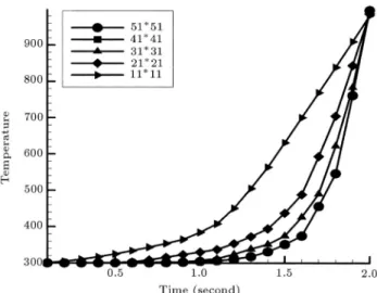
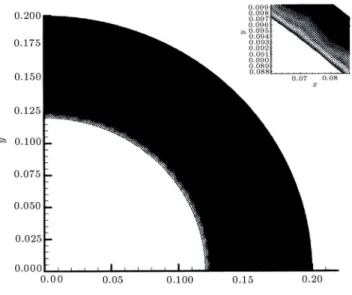
In order to investigate the grid size eect, ex-ploratory test runs were performed under various grid sizes to compute the temperature at the third sensor. The temperature history for these grids is plotted in Figure 1. The maximum changes in the temperature between the coarsest mesh (1111) and the nest mesh (5151) are within 85%. The results show that by increasing the neness of the grid to more than (41 41), no signicant changes appear in the temperature history. The nal computations were performed with (4141) grid points to maintain relatively moderate computing times in the nal calculations. A typical grid is shown in Figure 2a. The temperature contours att= 2 seconds are plotted and presented in Figure 2b. As seen from this gure, the thermal penetration depth of the heat ux is less than 3 mm. This is due to
Figure1. The temperature history of the point
Figure2a. A typical grid presentation att= 2 s.
Figure2b. The temperature contours and the thermal
penetration depth att= 2 s.
the eect of low thermal diusivity of the solid fuel (less than 210
;7 m2/s). It is worth noting that in a semi-innite at plate with no moving boundary and with the same physical properties as the test case, the temperature at the depth of 3 mm varies only by one degree centigrade after 2 seconds. In this problem, the eective mechanism of the heat ux penetration is the velocity of the surface. Thus, the sensitivity of the computational domain is very low to the variation of the surface temperature.
The comparison between the simulated and the computed surface temperatures for m = 0:1C is shown in Figure 3a. In Figure 3b, the computed and simulated temperatures at the positions where the thermocouples are located, are compared with each other. The computed results are in very good agreement with the simulated data. However, as can
Figure 3a. Computed and simulated temperature on the
moving surface.
Figure 3b. Temperature of the four thermocouples
adjacent to the moving boundary.
be seen clearly from Figure 3a, this is not the case for surface temperatures. A good agreement between the computed and simulated surface temperature exists up to t = 1:0 s. At this point, the computed surface temperature diers from the simulated one. This phenomenon should be studied in conjunction with Figure 3c. As can be seen, the number of the thermocouples left in the computational domain decreases with time, due to the receding of the surface. Therefore, when a thermocouple leaves the computa-tional domain, the next adjacent thermocouple is at a distance relative to the moving surface outside the thermal penetration depth. The receding boundary approaches the thermocouple causing the temperature variation to be felt by this sensor and the simulated and computed result coincides again.
Figure3c. The number of active thermocouple.
To investigate the inuence of the thermocouple's errors on the solution, the variance of the dierence between the simulated and the computed temperature of the moving surface, b = var(Tbc ;Tbs)
1=2, is obtained and plotted for dierent m, in Figure 4a.
Also, the mean value of the deviation between com-puted and simulated results, b = E(Tbc ;Tbs), is shown in Figure 4b. As seen from Figure 4a, the calculated variance increases with increasingm. This
is the obvious nature of the inverse heat conduction problem increased errors in thermocouple readings increases the errors in computing boundary temper-ature values. However, this gure shows that the method is applicable for moving boundary problems. For example, if K-type thermocouples, which have one degree centigrade normal error, are used, the error occurring in the solution will be approximately 10C. As can be seen from Figure 4b, the method
Figure4a. bversusm.
Figure4b. bversusm.
is unbiased for a small error value in temperature measurement.
The inuence of the thermal diusivity,, on the solution is investigated by examining the variation ofb
andbfor dierent, assuming constantm= 0:1C. As seen from Figure 5a, at low thermal diusivity, the variation of b is in the same order as the error of
sensors. However, after = 10;4 m2/s, a very sharp decrease in b is observed. The sharp decrease in b
is due to the fact that the thermal penetration depth is directly related to the thermal diusivity. As in-creases, the thermal penetration depth becomes larger, increasing the sensitivity of the adjacent thermocouple to the temperature of the moving surface. Increasing the value of to more than 10;4 m2/s, decreases the errors in the solution. From Figure 5b, it can be seen that the method is unbiased for large diusivity and relatively unbiased for small ones.
Figure5b. bversus diusivity.
Figure6a. Increment of temperature in each of iteration, jTbj.
Figure6b. Relative sum of square of errors, jEk
+1
;Ekj=Ek.
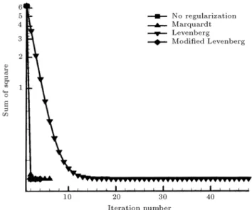
Figure 6c. Sum of square of errors,Ek.
To improve the convergence rate and the accuracy of the estimation, three regularization methods are used. In Figures 6a to 6c, the decrease in Tb,
the relative sum of the square of the errors and the sum of the square of the errors in each iteration, are shown. The Marquardt and Levenberg regularization methods under-relax the solution and, thereby, delay the convergence. No signicant changes are observed employing the modied Levenberg method. As can be seen from Figures 6a to 6c, the applied regularization methods do not enhance the accuracy of the obtained results. Therefore, the contribution of the regulariza-tion methods to overcome the ill-condiregulariza-tion of the mov-ing boundary inverse heat problems, is insignicant. As the mapping of the innite dimension to a nite dimension domain can act as a kind of regularization, the applied modied nite-element method, by itself, avoids the ill-condition problem associated with the moving boundary.
CONCLUSION
A exible hybrid method is presented for solving an inverse heat conduction problem with a moving bound-ary. Based on the moving nite element and transnite mapping properties, the method is developed for the cases with complex moving boundary conditions. The unique feature of the proposed algorithm is that the method can be used to treat any cases with unknown surface heat ux, surface temperature and heat transfer coecient on the moving surface. The applicability of the proposed method has been demonstrated in a case involving the burning of a homogenous solid fuel with unknown surface temperature on the receding boundary. The excellent correlation of the computed temperature histories and those measured at selected locations in the solid wall provides a clear indication
of the credibility of the proposed method. From the results, it appears that reasonably accurate estimation could be made, even when measurement errors are considered. The velocity of the receding surface on the formation of the thermal penetration depth and, hence, on the sensitivity of the sensors measuring the temperature, is recognized and discussed. Some oscillations in temperature readings are observed when a sensor is swept over by the thermal penetration depth and leaves the computational domain. Thus in online measurements of the boundary temperature, these oscillations should be omitted from the results. The variation of the thermal diusivity on the solution is also considered. The eect of dierent regularization methods on the convergence and accuracy of the solu-tion is investigated. It is shown that the employment of regularization does not have any signicant role in the convergence of the solution and the accuracy of the obtained results.
REFERENCES
1. Beck, J.V., Blackwell, B. and Clair, C.R.ST., Jr.,
Inverse Heat Conduction, John Wiley and Sons (1985). 2. Hensel, E.,Inverse Theory and Applications for
Engi-neering, Prentice Hall (1991).
3. Engl, H.W., Hanke, M. and Neubauer, A., Regulariza-tion of Inverse Problems, Kluwer Academic Publica-tion (1996.).
4. Isakov, V., Inverse Problems for Partial Dieren-tial Equations, Springer-Verlag Inc., New York, USA (1998).
5. Ozisik, M.N. and Orlande, H.R.B.,Inverse Heat Trans-fer: Fundamentals and Application, Taylor & Francis (2000).
6. Kakaee, A.H. and Farhanieh, B. \Investigation of dierent regularization parameters in an inverse heat conduction problem using nite element method",
International J. of Engineering Science,13(4), pp
173-190 (2002) .
7. Taler, J. and Zima, W. \Solution of inverse heat conduction problems using control volume approach",
Int. J. Heat & Mass Transfer, 42, pp 1123-1140,
Pergamon Press (1999).
8. Keanini, R.G. and Desai, N.N. \Inverse nite element reduced mesh method for predicting multidimensional phase change boundaries and nonlinear solid phase heat transfer",Int. J. Heat &Mass Transfer, 39, pp
1039-1049, Pergamon Press (1996).
9. Huang, C.H., Ozisik, M.N. and Sawaf, B. \Conjugate gradient method for determining unknown contactance during metal casting", Int. J. Heat Mass Transfer,
35(7), pp 1779-1786 (1992).
10. Keanini, R.G. and Desai, N.N. \Inverse nite element reduced mesh method for predicting multi-dimensional phase change boundaries and non-linear solid phase
heat transfer", Int. J. Heat Mass Transfer, 39(5), pp
1039-1049 (1996).
11. Woodbury, K.A. and Ke, Q. \A boundary inverse heat conduction problem with phase change for moisture-bearing porous medium", Inverse Problem in Engi-neering: Theory and Practice, 3rd Int. Conference on Inverse Problems in Engineering, June 13-18 (1999). 12. Xu, R. and Naterer, G.F. \Inverse method with heat
and entropy transport in solidication processing of materials",J. Material Processing Technology,112, pp
98-108 (2000).
13. Barth, T. \On unstructured grids and solvers",
VonKarman Inst. Lect. Series in Comp. Fluid Dynam-ics,3, pp 1-65 (1990).
14. Beck, J.V. \Non-linear estimation applied to the non-linear heat conduction problem", Int. J. Heat Mass Transfer,13, pp 703-716 (1970).
15. Tikhonov, A.N. \Regularization of incorrectly posed problems",Soviet Math. Dokl.,4, pp 1624-1627 (1963).
16. Phillips, D.L. \A technique for the numerical solution of certain integral equations of the rst kind",J. Assoc. Comput. Mach.,9, pp 84-97 (1962).
17. Levenberg, K. \A method for the solution of certain non-linear problems in least squares", Quart. Appl. Math.,2, pp 164-168 (1944).
18. Davies, M. and Whitting, I.J. \A modied form of Levenberg's Correction",Numerical Methods for Non-linear Optimization, Loostma, F.A., Ed., Academic Press, London, pp 191-201 (1972).
19. Marquardt, D.W. \An algorithm for least squares estimation of non-linear parameters", J. Soc. Ind. Appl. Math.,11, pp 431- 441 (1963).
20. Albert, M.R. and O'Neil, K. \Moving boundary-moving mesh analysis of phase change using nite elements with transnite mappings", Int. J. Numer. Meth. Engineering,23, pp 591-607 (1986).
21. Kakaee, A.H.,Solution of the Two Dimensional Navier Stokes Equations on Unstructured Triangular Meshes for Laminar Fluid Flow, M.Sc. Thesis, Sharif Univer-sity of Technology (1995).
22. Harrier, E. and Warner, G.,Solving Ordinary Dieren-tial Equations: Sti Problems, Springer Verlag (1991). 23. Golub, G.H. and Van loon, C.F., Matrix
Computa-tions, Johns Hopkins Univ. Press (1989).
24. Du, I.S., Erisman, A.M. and Reid, J.K., Direct Methods for Sparse Matrices, Clarendon Press, Oxford (1986).
25. Haber, R., Shepard, M.S., Abel, J.F., Gallagher, R.H. and Greenberg, D.P. \A general two dimensional graphical nite processor utilizing discrete transnite mappings",Int. J. Num. Meth. Engng.,17, pp
1015-1044 (1981).
26. Gordon, W.J. \Blending-function methods bivariate and multivariate interpolation and approximation",
27. Gordon, W.J. and Hall, C.A. \Construction of curvi-linear coordinate systems and application and approx-imation to mesh generation",Int. J. Num. Meth. Engng.,7, pp 461-477 (1973).
28. Hall, C.A. \Transnite interpolation and applications to engineering problems, in theory of approximation", Low and Sahney, Eds., Academic Press, pp 308-331 (1976).
29. Huang, C.H. and Yan, J.Y. \An inverse problem in predicting temperature dependent heat capacity per unit volume without internal measurements", Int. J. Numer. Meth. Engineering,39, pp 605-618 (1996).
30. Jarny, Y., Ozisik, M.N. and Bardon, J.P. \A general optimization method using adjoint equation for solving multidimensional inverse heat conduction", Int. J. Heat Mass Transfer,34, pp 2911-2919 (1991).
31. Press, W.H., Teukolsky, S.A., Vetterling, W.T. and Flannery, B.P., Numerical Recipes in FORTRAN: Art of Scientic Computing, Cambridge Univ. Press (1992).
32. Timnat, Y.M.,Advanced Chemical Rocket Propulsion, Academic Press (1987).