Eects of Unsteady Friction Factor on Gaseous Cavitation Model

Eects of Unsteady Friction Factor

on Gaseous Cavitation Model

M. Mosharaf Dehkordi

_{and B. Firoozabadi}

Abstract. The condition known as a water-hammer problem is a transient condition that may occur as a result of worst-case loadings, such as pump failures, valve closures, etc. in pipeline systems. The pressure in the water hammer can vary in such a way that in some cases it may increase and cause destruction to the hydraulic systems. The pressure in the water hammer can also be decreased to the extent that it can fall under the saturation pressure, where cavitation appears. Therefore, the liquid is vaporized, thus, making a two-phase ow. This pressure decrease can be as dangerous as the pressure rise. As a result of the pressure drop and vaporization of the liquid, two liquid regions are separated, which is referred to as column separation. In almost all standard methods for simulation of column separation, the steady friction factor was used, but in reality, the quantity of the friction factor is variable. In this work, the unsteady friction factor has been applied in the Discrete Gas Cavity Model (DGCM), which is a standard method of column separation prediction. Through comparisons with experimental data, results showed that applying the unsteady friction factor can improve the magnitude of the predicted duration shape and the timing of the pressure pulse in all of the case studies.

Keywords: Water-hammer; Cavitation; Discrete gas cavity model; Unsteady friction model; Method of characteristics.

INTRODUCTION

In a transient ow, a common concern of hydraulics engineers is to control the eect of the pressure wave, in order to protect relevant system components. Pressure waves are usually produced by the closure of a valve in simple systems. The pressure in hydraulic systems oscillates due to these pressure waves. In some cases, pressure reaches or drops below the vapor pressure and, therefore, cavitation occurs. Transient cavitation is an additional phenomenon accompanying the water-hammer. Cavitation can cause damage to the material of the pipes. The inuence of a pressure rise due to cavitation and pressure oscillation caused by water-hammer can be harmful to a pipe wall, as well as to its fatigue life. In order to improve the performance and reliability of systems, it is important to predict the onset and degree of cavitation taking place [1]. Fluid mixtures in hydraulic systems can be classied into ve groups:

1. School of Mechanical Engineering, Sharif University of Tech-nology, Tehran, P.O. Box 11155-956, Iran.

*. Corresponding author. E-mail: [email protected] Received 17 July 2008; received in revised form 20 May 2009; accepted 12 October 2009

1. Fully degassed liquid;

2. Fully degassed liquid with vapor; 3. Liquid with dissolved gas;

4. Liquid with dissolved and undissolved gas;

5. Liquid with dissolved and undissolved gas and vapor.

When the pressure reaches or drops below the vapor pressure of a liquid, the cavities grow very rapidly because of evaporation into the growing cavity. The process is called vaporous cavitation [1].

Cavitation can have a serious eect on pipeline systems. The accident at the Oigawa hydropower plant in 1950 in Japan is such an example, which was the result of column separation [2]. In that accident, three workers died. A fast valve-closure during maintenance caused an extreme high-pressure wave that split the penstock open. Therefore, a low pressure wave was generated causing cavitation and a portion of the pipeline was crushed due to the outer atmospheric pressure load. Jaeger et al. [3] reviewed the most serious accidents due to water-hammer and column separation. Many of the failures described were related to vibration and resonance [2].

In most industrial systems, a negligible amount of free and released gas in the liquid is assumed during column separation [4]. Two distinct types of column separation can be considered. The rst type is local vaporization with a large void fraction. A local vapor cavity may form in places such as a valve or in elevated regions of the pipe.

The second type of column separation is dis-tributed vaporous cavitation. In this type of column separation, the cavities may be extended over long sections of the pipe; the void fraction for the mixture of liquid and liquid-vapor bubbles is close to zero. As soon as a rarefaction wave progressively drops the pressure in an extended region of the pipe to liquid vapor pressure, distributed vaporous cavitation occurs. The collapse of a discrete vapor cavity and the movement of the shock wave front into a distributed vaporous cavitation region condense the vapor back to liquid. In transient events, the pressure oscillates; therefore, the pipeline systems may experience combined water-hammer and cavitation eects [5-7]. Several system parameters, including the type of transient regime (rapid closure of the valve and turbine load rejection), pipeline system properties (pipe dimensions, prole and position of valves) and hydraulic characteristics (velocity, pressure head, pipe wall friction, proper-ties of liquid and pipe walls) have important eects on the location and intensity of column separation; therefore, the modeling and laboratory testing of these phenomena are dicult. Practical implications of column separation led to intensive laboratory and eld research, starting at the end of the 19th century [4]. There are several research undertakings on a simple reservoir-pipeline-valve system. They showed that, when the cavities collapse at the valve, the pressure rise may or may not exceed the Joukowsky pressure rise, and cavities may form at the boundary or along the pipe [2,4].

There are dierent methods for the simulation of cavitation and column separation one of which is the Discrete Vapor-Cavity Model (DVCM) that is used in most commercial software packages for water-hammer analysis (such as HAMMER7) for simulating transient events in pipelines involving water column separation. Since the introduction of DVCM by Streeter [8], the DVCM may have generated unreal-istic pressure head spikes due to multicavity collapse. Kranenburg [9], Wylie and Streeter [7], Simpson and Bergant [10] and Brunone et al. [11] investigated the eects of multicavity collapse in column separa-tion. In an eort to improve the performance of the DVCM, several models were introduced by Wylie and Streeter [7] and Bergant and Simpson [6] as an alterna-tive to the discrete vapor-cavity model; Provoost and Wylie [12] introduced the discrete gas cavity model (DGCM).

In this paper, DGCM was modied by considering the unsteady friction factor, and the angle of the characteristic line in the Methods Of Characteristics (MOC) was corrected. The simulation was performed by a VC++ computer code, which can consider both steady and unsteady friction factors in the DGCM model.

Discrete Gas Cavity Model (DGCM)

As the pressure in the hydraulic system reaches or drops below the vapor pressure of the liquid, column separation occurs. As long as the pressure remains above the vapor pressure, with the absence of free gas in liquid, the wave speed remains constant. Whenever the pressure reaches or drops below the vapor pressure, vaporization occurs and the dynamic behavior of the system is changed; although the wave speed remains constant throughout the regions containing pure liq-uid [5].

There are several methods for simulating cavita-tion in transient events, such as the Discrete Vapor Cavity Model (DVCM) and the Discrete Gas Cavity Model (DGCM). In DGCM, for modeling the free gas distributed throughout the liquid in a homogeneous mixture, a free-gas lumped mass at computing sections is considered [5]. As a result of pressure variation, each isolated small volume of gas expands and contracts isothermally (for very small cavities). Between the computing sections, pure liquid is considered, and lumping the free gas at discrete locations has an eect on wave propagation speed that closely matches actual wave speed in the distributed mixture.

Unsteady Friction Models

The steady or quasi-steady friction terms are used in the standard water-hammer and column separation algorithms and software packages. For slow transient ows where the wall shear stress has a quasi-steady behavior, this assumption is reasonable. But, for rapid transients, experimental data have shown a signicant dierence when the computational results are com-pared to those of measurements [4]. The unsteady friction terms can be classied into six groups [13]: 1. The friction term is dependent on the instantaneous

mean ow velocity, V ;

2. The friction term is dependent on the instantaneous mean ow velocity, V , and instantaneous local acceleration, @V=@t;

3. The friction term is dependent on instantaneous mean ow velocity, V , instantaneous local accelera-tion, @V=@t, and instantaneous convective acceler-ation, V @V=@X.

4. The friction term is dependent on instantaneous mean ow velocity, V , and diusion, @2_V=@x2_. 5. The friction term is dependent on instantaneous

mean ow velocity, V , and weights for the past velocity changes, W () (Zielke model);

6. The friction term is based on the cross-sectional distribution of instantaneous ow velocity (2-D models).

The Zielke model [14] was analytically developed for the transient laminar ow. The unsteady part of the friction term is related to the weighted past velocity changes at the computational section. The Zielke model requires large computer storage, and several researchers have tried to improve computational eciency and/or extend its application to transient turbulent ow conditions.

The Brunone's model [15] is used in this pa-per, which is related to instantaneous local accelera-tion, @V=@t, and instantaneous convective acceleraaccelera-tion, V @V=@x.

MATHEMATICAL MODELS

Discrete Gas Cavity Model (DGCM)

In this scheme, it is assumed that between each com-puting section, there is pure liquid (without free gas) and a liquid phase with a constant wave speed occupy-ing the computational reach. The Discrete Gas Cavity Model (DGCM) allows gas cavities to form at com-putational sections in the method of characteristics. The DGCM is based on water-hammer compatibility equations, the continuity equation for the gas volume, and the ideal gas equation (isothermal process). The gas is assumed to behave isothermally, which is valid for tiny bubbles. Large bubbles and column separation tend to behave adiabatically. Figure 1 shows a section of the pipeline with a concentrated gas volume at computing sections. The perfect gas law is used to determine the volume of a constant mass of free gas in each computing section, which can be written in the following expression:

p

g 8g= MgRgT = p008; (1) in which T is temperature, Mgis mass of gas, Rgis gas constant, and 0is the void fraction at some reference pressure, p

0.

In most cases, we deal with free air in water. In these cases we use the hydraulic-grade line convenient (Figure 1).

p

g = lg(H z H); (2)

in which the hydraulic-grade line elevation, H, and the elevation of the pipeline, z, are measured from the same

Figure 1. Hydraulic-grade line for the pipeline [5].

reference datum. Since 8, the volume of mixture in a pipeline reach is a constant, Equation 1 may be used to determine the volume of gas at each section for initial conditions and for each time step:

80 g= p

008

p

g =

C3

H z H; (3)

in which C3 = p008=lg.

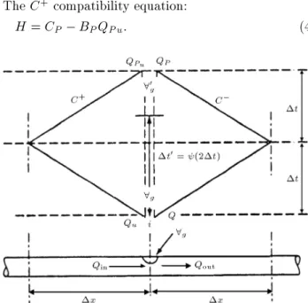
Figure 2 shows a staggered grid of characteristics when the gas volume is at an interior section in the pipeline.

The equations needed to solve the variable at each time step are:

The C+_{compatibility equation:}

H = CP BPQP u: (4)

Figure 2. Staggered grid of characteristics at an interior section in the pipeline.

The C compatibility equation:

H = CM BMQP; (5)

in which the coecients CP, BP, CM and BM are: CP = Hi 1 BQi 1;

BP = B + RjQi 1j; CM = Hi+1 BQi+1; BM = B + RjQi+1j

in which B = a=gA and R = fx=2gDA2_. The continuity equation at the gas volume is:

d8g

dt = Qout Qin: (6)

By using the weighting factor in the time direction (as shown in Figure 2), which is dened in the form:

= t0

2T; 0:5 < 1; (7)

Equation 6 is integrated and yields: 80

g= 8g+ 2t

[ (QP QP u) + (1 )(Q Qu)]; (8) in which 2t = 2x=a is time step, 80

g and 8g are gas volume at the current time and 2t earlier, respectively.

Substitution of Equations 4 to 6 into Equation 8 leads to:

(H z H)2+ 2B1(H z H) C4= 0; (9) in which:

B1= Bz(BPCM + CPBM) + B2BPBMB+ (z + H)=2; C4= C3BPBMB2=(t ); B2= 0:5=(BM + BP);

B = b8g=(2t) + (1 )(Q Qu)c= :

This standard quadratic equation has the solution: H z H= B1(1 +

p

1 + BB) if B1<0; (10) H z H= B1(1

p

1 + BB) if B1>0; (11)

in which BB= C4=B21. Equations 5 and 6 are used to nd QP u and QP, and Equation 8 is used to nd 80g.

A straightforward linearization of these equations, for the condition of jBBj << 1 is used to avoid yielding inaccurate results due to inaccuracies in the numerical evaluation of the radical.

H z H= 2B1 _2BC4

1 if B < 0; (12) H z H= _2BC4

1 if B1> 0: (13) Thus, Equations 12 and 13 are used when jBBj is small (less than 0.001), and Equations 10 and 11 are used in all other cases.

To control the numerical oscillations that appear during the simulation of a transient, the weighting factor, , is used [5]. Although the weighting factor, , can take on values between 0 and 1.0, a practical range is 0.5-1.0. For values less than 0.5, the results are unstable, and at = 1 there is minimum numerical oscillation [5].

Bergant et al. [16] showed that the value of void fraction, 0, has signicant eects on the pressure wave shape and timing for a very low gas void fraction; the DGCM model results perfectly matched with the re-sults of standard water hammer model (in the absence of cavitation) It is also depicted that larger amounts of free gas have more eect on results in shape and timing. Therefore, the DGCM model can be successfully used for simulation of vaporous cavitation by utilizing a very low gas void fraction (0 10 7). Another factor that has a serious eect on results in shape and timing is the ow situation. Bergant considered two distinct ow situations:

1. Distributed free gas at all computational sections; 2. A trapped gas pocket at the midpoint of the

pipeline system (shown in Figure 3). In the present work, DGCM was used by considering a very low gas void fraction and distributed free gas at all computational sections.

Unsteady Friction Factor Models

In most software packages, the steady state friction factor is used for water-hammer analysis. For consid-ering the eects of unsteady friction on water-hammer or column separation, friction factor f in Equations 4 and 5 can be expressed as the sum of a quasi-steady part, fq, and an unsteady part, fu, i.e. f = fq+ fu. It should be mentioned that by setting fu = 0 the steady friction model, fq, is computed by updating the Reynolds number at each new computation, based on Vakil and Firoozabadi [13], who used an unsteady friction factor in water-hammer without cavitation.

Here, the Brunone model was used to consider the unsteady friction factor. The Brunone model relates the unsteady friction part, fu, to the instantaneous local acceleration, @V=@t, and instantaneous convec-tive acceleration, V @V=@x; Vitkovsky deduced a new formulation based on Brunone's model [15]:

f = fq+k D A_QjQj

@Q

@t + a sign(Q)

@Q_@x; (14) in which:

sign(Q) = f+1 for Q 0 and 1 for Q < 0g: The Brunone friction coecient k can be predicted either empirically or analytically [17]. The analytical denition of k using Vardy and Brown's shear decay coecient, C_{, is used in this paper:}

k = p

C

2 ; (15)

in which: C₌

(

0:00476 for laminar ow 7:41

Relog(14:3=Re0:05) for turbulent ow:

(16) A rst-order approximation for the friction term, i.e. f:Qt tjQt tj:x=(2gDA2), is used in Equations 4 and 5 when using the Brunone model.

Characteristic Equation in DGCM with Unsteady Friction Term

Water hammer equations include the continuity equa-tion and equaequa-tions of moequa-tion with assumpequa-tions, such as one-dimensional ow, steady friction term and no-column separation. Neglecting small terms in compar-ison with other terms are as follows [17]:

L1= @H_@t + a 2 gA

@Q

@x = 0; (17)

L2= @H_@x +_gA1 @Q_@t +_2gDAfQjQj₂ = 0: (18)

For considering the eects of unsteady friction in DGCM, substitution of Equation 14 into Equation 18 leads to:

L2= @H_@x +_gA1 @Q_@t +f_2gDAq QjQj₂ + k

@Q

@t + a A @Q @x ; (19) in which: A= (

1 for Q@Q=@x < 0 +1 for Q@Q=@x > 0

Equations 2 and 12 are combined linearly using un-known multiplier in the form of L2 + L1 = 0, and using a material derivative for H(x; t) and Q(x; t) which leads to:

dx dt =

1 =

aAk + a2

1 + k ; (20)

Equation 20 is solved for an unknown multiplier: 1;2= k_2aA _2a1 (k + 2): (21) The procedure is similar to the MOC in a standard water-hammer, thus, by integrating along characteris-tic lines, the nite dierence equation is determined. Considering the value of shows that, by using the unsteady friction coecient, the angle of characteristic lines is changed and, thus, coecients CP, BP, CM and BM are changed and must be updated. By using recent values of these coecients, Equations 5 to 14 are computed.

Updating Brunone Friction Coecient k The analytical denition of k using Vardy and Brown's shear decay coecient, C_{, that is used in this paper,} is shown in Equations 15 and 16. In the present work, the Reynolds number is determined by using the local discharge in each computing section (node). However, in cases of cavitation, there are two local discharges in each computing section (inow and outow) and, therefore, there are two distinct methods for updating the local Reynolds number and the Brunone friction coecient. With respect to the two forms of denition of the Vardy shear decay coecient (Equation 16), whenever the local Reynolds number is not zero, the Brunone coecient is updated. Both of these methods were studied. In Equation 19, A was introduced as follows:

A= (

1 for Q@Q=@x < 0 +1 for Q@Q=@x > 0

To determine A, Q@Q=@x must be calculated at each computing section, thus along the C+ _{characteristic} line:

(Qu)i;t:(Qu)i;t_xQi 1;t; (22) and along the C characteristic line:

Qi;t:(Qu)i+1;t_x Qi;t: (23) TEST CASE

To verify the present model, results were compared with the experimental data, as well as with other numerical results of column separation simulation in hydraulic systems.

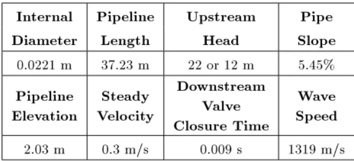
Bergant and Simpson [4] designed and con-structed exible laboratory apparatus for investigat-ing water hammer and column separation events in pipelines. Their apparatus is comprised of a straight sloping copper pipe connecting two pressurized tanks (Figure 3). The pipe slope is constant at 5.45% [4]. Water hammer events in the apparatus are initiated by rapid closure of the ball valve. The properties of this system are shown in Table 1.

RESULTS AND DISCUSSION Dierent Initial Velocities

Results for two distinct ow velocities in an upward sloping pipe (shown in Figure 3; V0 = 0.3 or 1.4 m/s) and a constant upstream end reservoir head (Tank 2; HT;2 = 22.0 m) are presented here. The numerical prediction and measured piezometric heads at the downstream end valve, H;1, and at the mid-point, Hmp, (Figure 3) were calculated for a low-velocity case (V0 = 0.3 m/s). A comparison between experimental results [4] and the present work for the steady and unsteady friction DGCM can be seen in Figures 4 and 5, respectively.

Table 1. Properties of the system. Internal Pipeline Upstream Pipe Diameter Length Head Slope

0.0221 m 37.23 m 22 or 12 m 5.45% Pipeline Elevation Steady Velocity Downstream Valve Closure Time Wave Speed 2.03 m 0.3 m/s 0.009 s 1319 m/s

It should be mentioned that Equations 15 and 16 show that the Brunone friction coecient depends on Reynolds number. In case of cavitations, there are two ows in each computational node (inow and outow), therefore, there are two dierent methods (two Reynolds numbers) for updating k in the unsteady friction model. In Figures 5 to 7, k in each node is updated by using the outow.

The valve closure generates the water-hammer head, H;1 = 62.5 m, and subsequent column sepa-ration at the valve in a time of 0.0662 seconds. The maximum measured head, Hmax;;a = 95.6 m, occurs in a time of 0.1842 seconds as a narrow short-duration pressure pulse. The magnitude of the short-duration pressure pulse predicted by DGCM is Hmax;;1 = 100.36 m (present work: steady friction) and Hmax;;1 = 101.9 m from Bergant and Simpson simulations [4]. The unsteady friction DGCM (present work) pressure is predicted as Hmax;;1 = 100.1 m. A comparison of the results of all studied models and experimental results [4] is shown in Table 2. A comparison of pressure heads and times of occurrence is done for 4 points (these points are shown in Figure 4a).

As can be seen from Table 2, at all points the unsteady friction DGCM predicted by the present work has good agreement with the measured values reported by [4]. It is also evident that the unsteady friction model can improve the time and shape of oscillations.

Figure 6 shows a comparison between the present work and measured values of the downstream valve head for an inlet velocity of V0 = 1.4 m/s. The maximum head at the valve is the water hammer head generated at a time of 2L=a after valve closure. The wa-ter hammer head predicted by DGCM (steady friction and unsteady friction terms) matches the measured head. In this case, using an unsteady friction term can predict a better result in shape and timing compared with the steady friction term.

Dierent Reservoir Static Heads

The results for two dierent static heads in the up-stream end reservoir (HT;2= 12.0 or 22.0 m) and initial velocity (V0 = 0:3 m/s) are compared in Figures 4 to 7. A valve closure for HT;2= 12.0 m generates column separation with a wide short-duration pressure pulse (Figure 7), which is compared to column separation with a narrow short- duration pressure pulse (Figures 4 and 5). The decrease of static head at the identical initial ow velocity results in the reduced amplitude of a short-duration pressure pulse (lower amplitude reservoir wave) and more intense cavitation [4]. Both numerical models accurately predict the magnitude of the wide short duration pressure pulse and the duration of the rst cavity at the valve in comparison with the

Figure 4. Comparison between measurements [4] and DGCM, with steady friction term.(a) and (b) Present Work, (c) and (d) Bergant and Simpson's work [4] (V0 = 0.3 m/s).

Figure 5. Comparison between present work (unsteady friction DGCM) and measured results (V0 = 0.3 m/s). (a) Heads

in downstream valve; (b) Mid-point of pipeline.

experimental data (Figures 7). As can be seen, the unsteady friction factor improves the results in the shape and timing of oscillations.

As shown in Table 3, the unsteady friction DGCM has better prediction than the DGCM model in agree-ment with measureagree-ment data [4].

Dierent Methods for Updating Brunone Friction Coecient

In this work, the Brunone coecient, k, is updated by using the local Reynolds number. In each node, as cavitation occurs, there are two dierent discharges

Table 2. Comparison of water-hammer head, maximum head, peak head, and time corresponding to peaks calculated from dierent numerical models and experimental data in downstream valve.

Point No. (as Shown in

Figure 4a)

1 2 3 4

Method of Evaluation

H;1 (m)

(1st Peak)

Time (s)

Hmax;;1 (m)

(2nd Peak)

Time (s)

H;1 (m)

(4th Peak)

Time (s)

H;1 (m)

(5th Peak)

Time (s) Measured Values

[4] 62.50 0.0662 95.6 0.1842 60.51 0.3794 48.82 0.4945 Simulation DGCM

[4] 62.42 0.0591 101.9 0.1833 51.339 0.3661 51.03 0.4792 DGCM with

Steady Friction (Present Work)

62.43 0.0585 100.36 0.1834 46.174 0.3669 44.96 0.4798

DGCM with Unsteady Friction

(Present Work)

62.43 0.0621 100.1 0.1841 55.84 0.3739 48.71 0.4868

Figure 6. Comparison of heads in downstream valve for DGCM (a) and unsteady friction DGCM (b) with measured results (V0 = 1.4 m/s).

Figure 7. Heads in downstream valve; comparison between measured results [4] and predicted values by the present work. (a) Steady friction DGCM; (b) Unsteady friction DGCM; HT;2= 12.0 m.

Table 3. Comparison of peak head, and time corresponding to peaks calculated from dierent numerical models and experimental data in downstream valve, HT;2= 12:0 m.

Point No. (as Shown in

Figure 4a)

1 2 3 4

Method of Evaluation

H;1 (m)

(1st Peak)

Time (s)

H;1 (m)

(2nd Peak)

Time (s)

H;1 (m)

(3rd Peak)

Time (s)

H;1 (m)

(4th Peak)

Time (s) Measured Values

[4] 51.73 0.0135 53.48 0.2181 54.25 0.370 48.60 0.481 DGCM with

Steady Friction (Present Work)

51.62 0.0141 53.16 0.2116 53.95 0.359 53.50 0.494

DGCM with Unsteady Friction

(Present Work)

51.62 0.0141 54.07 0.2187 53.99 0.367 51.20 0.487

Qin and Qout (as shown in Figure 2), so the Reynolds number, Re = V D= = 4Q=D, can be calculated using two dierent velocities. Therefore, there are two dierent methods for updating the Reynolds number.

In the rst method, the Brunone coecient, k, was updated, using the outow of each node for calculation of the Reynolds number. In the second method, the local Reynolds number and the Brunone coecient, k, were updated using inow.

Figures 8, 9a and 10a show the results of unsteady friction DGCM (inow) compared to the measure-ments [4] for a dierent initial velocity (V0 = 0.3 or 1.4 m/s) and dierent upstream heads (HT;2= 12.0 or 22.0 m).

Figures 9b, 10b and 11 show comparisons of all numerical models (that were studied) with mea-surements results. These gures show that using the unsteady friction model can improve the result, compared to the measurement, in most cases, but

the form of applying the unsteady friction term in MOC and updating the Brunone coecient are very important. In all conditions studied, unsteady friction DGCM (that uses outow for calculation of the local Reynolds number) has had the best results (between all methods that were studied) compared to the mea-surement results; however, more studies are required to show the validity of this statement.

Figures 9b, 10b and 11 show that in some cases, the unsteady friction model predicts higher pressure peaks compared to steady friction models, but in general, the results of unsteady friction models (both inow and outow) are better than those of the DGCM model in timing. The problem (prediction of higher peaks) in the outow model is less than that of the inow model; therefore, the unsteady friction DGCM (using outow for calculation of the local Reynolds number) is the best model for simulation of the column separation studies.

Figure 8. Comparison of heads for unsteady friction DGCM (inow) (a) in downstream valve and (b) for mid-point of pipeline with measured results; HT;2 = 22.0 m, V0 = 0.3 m/s.

Figure 9. Comparison of heads in downstream valve for unsteady friction DGCM (inow) (a) and all studied methods (b) with measured results; HT;2 = 22.0 m, V0 = 1.4 m/s.

Figure 10. Comparison of heads in downstream valve for unsteady friction DGCM between inow (a) and outow (b) with measured results; HT;2 = 12.0 m, V0 = 0.3 m/s.

Figure 11. Comparison of heads for all studied methods (a) in downstream valve and (b) mid-point of pipeline with measured results; HT;2= 22.0 m, V0 = 0.3 m/s.

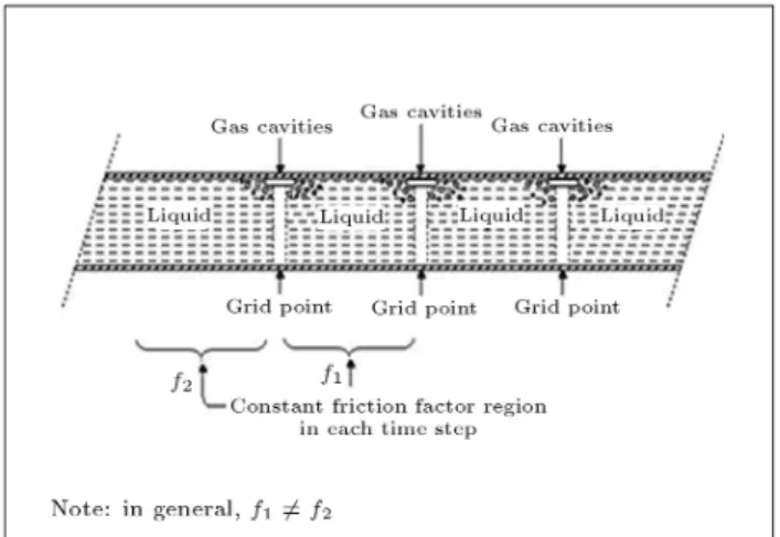
The velocity proles have greater gradients in an unsteady condition, which results in higher energy dissipation compared with the steady condition. The results show that the unsteady friction factor has some uctuations after the occurrence of each pressure peak, especially peak numbers 2, 3 and 4, which are shown in Figure 4a. Furthermore, in each time the values of the unsteady friction term are higher than the steady term, which is why it can predict a better agreement with experimental data. As far as we are concerned, the sound velocity and friction factor between two adjacent nodes are assumed to be constant; in other words, although there may be several friction factors, the friction factor between two adjacent computational nodes is constant. Figure 12 can clarify this point.

Finally, mesh independency was investigated and the results were independent of grid size.

CONCLUSION

The performance of the Brunone unsteady friction model has been tested for the DGCM for simulation of simple reservoir-pipeline-valve systems, including a test case. A comparison of two variations of the discrete vapor cavity model has been presented. The example presented shows that an unsteady friction model (modied Brunone's model) is able to predict a better result compared with measurements. These results clearly indicate the dependence of k on the Re number and the form of updating of this coe-cient on the shape of the results. The modication of k with the local Reynolds number is the key to producing an improved prediction for two-phase transient ows. Further work is required to establish an appropriate k particularly for a case of two-phase ow.

Figure 12. The variations of friction factors in pipeline in each time step.

NOMENCLATURE

a water hammer wave speed

A pipe area

C+ _{positive characteristic equation} C negative characteristic equation C _{Vardy's shear decay coecient} D pipe diameter

fq Darcy-Weisbach friction factor g gravitational acceleration

H barometric head Hi piezometric head H vapor pressure head

k Brunone's friction coecient L pipe length

N number of reaches in pipeline Q discharge at downstream side of

computational section

Qu discharge at upstream side of computational section

p

0 reference pressure p _{absolute pressure} Re Reynolds number V D= Tc valve closure time

V ow velocity or velocity at downstream side of vapor cavity

Vcav vapor cavity volume Zi elevation of pipe section

multiplier in characteristics method liquid density

t time step

x reach length weighting factor Subscripts

i node number

mp mid-point node Abbreviations

DVCM Discrete Vapor Cavity Model MOC Method Of Characteristics REFERENCES

1. Shu, J.J. \Modeling vaporous cavitation on uid tran-sients", International Journal of Pressure Vessels and Piping, 80, pp. 187-195 (2003).

2. Bergant, A. and Simpson, A.R. \Water hammer with column separation: A historical review", Journal of Fluids and Structures, 22, pp. 135-171 (2006).

3. Jaeger, C., Kerr, L.S. and Wylie, E.B. \Water hammer eects in power conduits", Proceedings of the Interna-tional Symposium on Water Hammer in Pumped Stor-age Projects, ASME Winter Annual Meeting, Chicago, USA, pp. 233-241 (1965).

4. Bergant, A. and Simpson, A.R. \Pipeline column separation ow regimes", ASCE Journal of Hydraulic Engineering, 125(8), pp. 835-848 (1999).

5. Wylie, E.B. and Streeter, V.L., Fluid Transients in Systems, Prentice-Hall, Englewood Clis (1993). 6. Simpson, A.R. and Bergant, A. \Numerical

com-parison of pipe column-separation models", ASCE, Journal of Hydraulic Engineering, 120, pp. 361-377 (1994).

7. Wylie, E.B. and Streeter, V.L. \Column separation in horizontal pipelines", Proceedings of the Joint Sympo-sium on Design and Operation of Fluid Machinery, 1, IAHR/ASME/ASCE, Colorado State University, Fort Collins, USA, pp. 3-13 (1978).

8. Streeter, V.L. \Transient cavitating pipe ow", ASCE Journal of Hydraulic Engineering, 109(HY11), pp. 1408-1423 (1983).

9. Kraneburg, C. \Transient cavitation in pipelines", Ph.D. Thesis, Delft University of Technology, Dept. of Civil Engineering, Laboratory of Fluid Mechanics, Delft, The Netherlands (1974).

10. Simpson, A.R. and Bergant, A. \Developments in pipeline column separation experimentation", IAHR, Journal of Hydraulic Research, 32, pp. 183-194 (1994).

11. Brunone, B., Golia, U.M. and Greco, M. \Eects of two-dimensionality on pipe transients modeling", Journal of Hydraulic Engineering, 121(12), pp. 906-912 (1995).

12. Proovost, G.A. and Wylie, E.B. \Discrete gas model to represent distributed free gas in liquids", Proceed-ings of the Fifth International Symposium on Wa-ter Column Separation, IAHR, Obernach, Germany, Also: Delft Hydraulics Laboratory, Publication No. 263 (1982).

13. Vakil, A. and Firoozabadi, B. \Eect of the unsteady friction models and friction-loss integration on the transient pipe ow", Scientia Iranica, 13(3), pp. 245-254 (2006).

14. Zielke, W. \Frequency-dependent friction in transient pipe ow", Journal of Basic Engineering, 90(1), pp.109-115 (1968).

15. Brunone, B., Karney, W., Mecarelli, M. and Ferrante, M. \ Velocity proles and unsteady pipe friction in transient ow", Journal of Water Resources Planning and Management, 126(4), pp. 236-244 (2000). 16. Bergant, A., Vithovsky, J. and Simpson, A.R.

\Devel-oping in unsteady pipe ow friction modeling", Journal of Hydraulic Research, 39(3), pp. 249-257 (2001). 17. Bergant, A. and Simpson, A.R. \Cavitation inception

in pipeline column separation", Proceedings of the 28th IAHR Congress, Graz, Austria, CD-ROM (1999).