Prediction of Longitudinal Dispersion
Coecient in Natural Channels
Using Soft Computing Techniques
S. Adarsh
1Abstract. Accurate estimate of longitudinal dispersion coecient is essential in many hydraulic and environmental problems such as intake designs, modeling ow in esturies and risk assessment of injection of hazardous pollutants into river ows. Recent research works show that in the absence of knowledge about explicit relationships concerning longitudinal dispersion coecient and its inuencing parameters, data driven techniques can be used to predict it with reasonable degree of accuracy. In this paper, the usefulness of Support Vector Machines (SVM) and Genetic Programming (GP) are examined for predicting longitudinal dispersion coecient in natural channels. The hydraulic variables such as ow depth (H), ow velocity (U) and shear velocity (u) along with the width of channel (B) are used
as input variables to predict longitudinal dispersion coecient (Kx). The performance evaluation based
on multiple error criteria conrm that GP shows remarkably good performance in capturing non-linear relationship between the predictors and predictant in the estimation of longitudinal dispersion coecient when compared with empirical approaches, the traditional Articial Neural Networks (ANN) and SVM. Hence GP can be used as an ecient computational paradigm in the prediction of longitudinal dispersion coecient in natural channels.
Keywords: Longitudinal dispersion coecient; Natural channels; Articial neural networks; Support vector machines; Genetic programming.
INTRODUCTION
Disposal of euent from industrial factories or acci-dental disposal of contaminants into natural channels like streams and rivers will deteriorate the quality of water due to lack of proper mixing. Pollution of natural water bodies has received wide attention among the re-searchers recently, as proper water quality management is essential for public health and for preserving natural water bodies. When the euents or contaminants are discharged into a river, it undergoes stages of mixing during the transportation to downstream by the river ow. The euent may get dispersed longitudinally, transversely and vertically by advective and dispersive process. Ability of river and other open channel ows in dispersing additive materials in longitudinal and transverse and vertical directions is described by
1. Department of Civil Engineering, TKM College of Engineer-ing Kollam- 691 005, Kerala, India. E-mail: adarsh lce@ yahoo.co.in
Received 14 February 2010; received in revised form 6 June 2010; accepted 16 August 2010
the dispersion coecients Kx, Ky and Kz,
respec-tively. Once the cross sectional mixing is complete, the process of longitudinal dispersion becomes the most important mechanism [1]. Thus, to know the fate of contaminant transport, the precise estimation of longitudinal dispersion coecient is required [2,3]. Accurate estimate of longitudinal dispersion coecient is required in many practical problems such as intake designs, modeling ow in esturies and risk assess-ment of injection of hazardous pollutants into river ows [4,5]. Taylor introduced longitudinal dispersion coecient as a measure of 1D dispersion in laminar and turbulent pipe ows [6,7]. Elder extended the dispersion in pipes to the mixing in an innitely wide channel and concluded that vertical velocity gradient is the main governing mechanism behind mixing [8]. Fischer attributed that the velocity heterogeneity is the underlying mechanism behind mixing [9]. He proposed an integral expression for determining the longitudinal dispersion coecient [9].
Later on, a number of investigators have proposed empirical equations based on experimental and eld
data for predicting longitudinal dispersion coecient, some among them are mentioned in [1]. However such equations are valid only in their calibrated and tested range of ow. Tayfur and Singh [10], Torpak and Cigizolu [11] used Articial Neural Network (ANN) as a tool for estimating longitudinal dispersion co-ecient. Toprak and Savci [12] applied fuzzy logic for prediction of longitudinal dispersion coecient in natural channels. Recently, Madvar et al. [13] proposed an Adaptive Neuro-Fuzzy Inference System (ANFIS) for the prediction of longitudinal dispersion coecient. Tayfur [14] applied Genetic Algorithm (GA) to predict longitudinal dispersion coecient in natural channels in an optimization framework. ANN has some inherent drawbacks such as slow convergence, less generalizing performance, arriving at local minimum and overtting problems [15]. After a detailed investigation of dierent empirical approaches, Madaver et al. [13] reported that these methods show varying degree of accuracy in the estimation of longitudinal dispersion coecient in natural channels. This opens the scope for the search for an ecient computational intelligence paradigm for accurate estimation of longitudinal dispersion co-ecient in natural channels. In this study, Support Vector Machines (SVM) and Genetic Programming (GP) are applied as alternative data driven techniques (soft computing techniques) for estimating longitudinal dispersion coecient in natural channels.
THEORETICAL BACKGROUND
The one-dimensional (1-D) Fickian type dispersion equation which is derived by Taylor [6] has been widely used to obtain reasonable estimates of the rate of longitudinal dispersion. The 1-D dispersion equation is: @Co @t + u @Co @x
= Kx
@2C
o
@x2
; (1)
where Co is the concentration average in section, u is
longitudinal average velocity, t is time, x is longitudinal direction in ow stream. Fischer [9] proposed a triple integral expression for estimation of longitudinal dispersion coecient in the following form:
Kx= A1
Z B
0 hu 0Z y
0
1 "th
Z y
0 hu
0dydydy; (2)
where A is the cross section area of ow, B is the top width of water surface, h is the local depth of ow in any transverse point, u0 is deviation of depth
averaged ow velocity from the cross sectional mean velocity, y is the transverse location from left bank and "tis transverse mixing coecient. It is noted that
Equation 2 is a basis for several empirical equations proposed for the determination of Kx. Fischer et al. [3]
suggested the following equation for determination of "t:
"t= 0:15Hu; (3)
where H is the average depth of ow of the cross section, u is the shear velocity and is given by u =
p
gHSf in which Sf is the slope of total energy line.
Fischer et al. [9] developed the following equation to predict Kx, which is a simplied form of Equation 2:
Kx= 0:011U 2B2
Hu ; (4)
where U is cross sectional average ow velocity. Seo and Cheong [1] used dimensional analysis and a non-linear multiple regression method to derive an expression for Kx. Deng et al. [16] followed a more
the-oretical approximation of Equation 2. They developed mathematical expressions for the lateral distribution over the ow depth, deviation of local velocity from mean velocity and transverse mixing coecient and substituted in Equation 2. By using 81 sets of measured data from 30 rivers in United States, Kashepour and Falconer [17] developed two models for predicting longitudinal dispersion coecient in rivers. These equations were developed by considering the hydraulic and geometric parameters by using dimensional and regression analyses.
SUPPORT VECTOR MACHINES
Support Vector Machine (SVM) is a relatively recent addition to the family of soft computing techniques evolved from the concept of statistical learning theory explored by Boser et al. [18]. SVM performs the regression by using a set of non-linear functions that are dened in a high dimensional space. SVM has been used to solve non-linear regression problems by risk minimization where the risk is measured using Vapnik's accuracy intensive loss function (") [19]. SVM uses a risk function consisting of the empirical error and a regularization term which is derived from the Structural Risk Minimization (SRM) principle. More details on SRM can be found in Cortes and Vapnik [20]. Considering a set of input-output pairs [(x1, y1), (x2,
y2) (xl, yl)] 2 RN, y 2 r as training dataset, where
x is the input, y is the output, RN is the N-dimensional
vector space and r is the one dimensional vector space. In this problem x = [B; H; U; u] and y = [Kx].
The intension of SVM is to t a function that can approximately predict the value of output on supplying a new set of predictors (input variables).
The "-intensive loss function can be described as follows:
otherwise:
L"(y) = jf(x) yj ": (6)
This denes an "-tube so that if the predicted values is within the tube, the loss is zero, otherwise the loss is equal to the absolute value of the deviation minus ". This concept is depicted in Figure 1.
SVM attempts to nd a function f(x) which tries to t a given dataset keeping the deviation from the actual output `"' as at as possible.
Consider a linear function of the following form: f(x) = (w:x) + b; w 2 RN; b 2 r; (7)
where w is an adjustable weight vector, and b is the scalar threshold. Fitness means the search for a small value of `w'. It can be represented as a minimization problem with an objective function comprising the Euclidian norm as follows:
Minimize: 1
2kwk2; (8)
subject to:
yi [(w:xi) + b] "; i = 1; 2; 3 l; (9)
[(w:xi) + b] yi "; i = 1; 2; 3 l: (10)
Some allowance for errors (") may also be introduced. Two slack parameters and have been introduced to
Figure 1. The "-tube and slack variable () in SVM.
penalize the samples with error more than `"'. Thus the infeasible constraints of the optimization problem are eliminated. The modied formulation takes the form: Minimize:
1
2kwk2+ C
l
X
i=1
(i+ i); (11)
Subject to:
yi [(w:xi) + b] " + i; i = 1; 2; 3 l; (12)
[(w:xi) + b] yi " + i; i = 1; 2; 3 l; (13)
i 0; i 0; i = 1; 2; 3; l: (14)
The constant 0 < C < 1 determines the trade-o between the atness of f(x) and the amount upto which the deviations larger than `"' are tolerated [21]. The above optimization problem is solved by Vapnik [22] using Lagrange Multiplier method. The solution is given by:
f(x) =XM
i=1
(i i)(xi:x) + b;
where: b =
1 2
w:(xr+ xs); (15)
where xsand xr are known as support vectors and M
is the number of support vectors.
Some Lagrange multipliers (i, i) will be zero,
which implies that these training solutions are irrele-vant to the nal solution (known as sparseness of the solution). The training objects with non zero Lagrange multipliers are called support vectors. When linear regression is not appropriate, input data have to be mapped into a high dimensional feature space through non linear mapping and the linear regression needs to be performed in the high dimensional feature space [18]. The mapping of input data onto the feature space can be done by . The dot product between (xi)
and (xj) is computed as a linear combination of the
training points. The concept of non-linear mapping is depicted by Figure 2.
The functions which satises Mercer's theorem can be used for tting the data reported in Boser et al. [18]. Polynomial functions, Radial Basis Func-tion (RBF) and splines are the most commonly used functions for data tting using SVM. Recently, SVM is successfully applied to many problems in water resources and environmental problems [23-25].
Figure 2. Concept of non-linear regression using SVM.
GENETIC PROGRAMMING
The evolutionary computational techniques may be the better alternatives for solving regression problems as they follow an optimization strategy with progressive improvement towards the global optima. They start with possible trial solutions within a decision space and the search is guided by genetic operators and the principle of `survival of the ttest' [26]. Genetic Algorithm (GA) is one of the most popular and powerful evolutionary optimization techniques [26,27], but it cannot be used to evolve complex models such as equations. This limitation is overcome by Genetic Programming (GP) introduced by Koza [28]. GP is an automatic programming technique for evolving computer programs to solve, or approximately solve, problems [28]. GP, which is basically an optimization paradigm, can also be eectively applied to the Genetic Symbolic Regression (GSR). GSR involves nding a mathematical expression in symbolic form relating nite values of set of independent variables (xi) and
a set of dependent variables (yi) [29]. GP is a
member of the Evolutionary Algorithm (EA) family, and works on Darwin's natural selection theory in evolution. Here, a population is progressively improved by selectively discarding the not-so-t population and breeding new children to form better populations. Like other evolutionary algorithms, the solution is started with a random population of individuals (equations or computer programs). Each possible solution set can
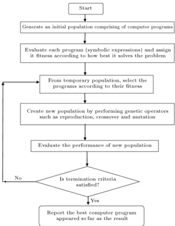
be visualized as a `parse tree' comprising the terminal set (input variables) and functions (generally operators such as +, , , =, logarithmic or trigonometric). The `tness' is a measure of how closely a trial solution solve the problem. The objective function { the minimization of error between estimated and observed value { is the tness function. The solution set in a population associated with the \best t" individuals will be reproduced more often than the less t solution sets. It iteratively transforms a population of computer programs into a new generation of programs by apply-ing analogs to naturally occurrapply-ing genetic operators like reproduction, mutation and crossover. The dierent genetic operations can be found in detail in [28]. The basic procedure of GP is presented as a ow chart in Figure 3.
In the recent years, GP is eectively applied to solve a wide range of water resources problems [29-33]. GP can evolve an explicit equation or equivalent com-puter program relating the input and output variables which is a more understandable depiction of the cause-eect process. A program-based approach is adopted for the present study.
DATASET USED FOR MODELING
The development of mathematical model to predict longitudinal dispersion coecient and its validation
Table 1. Statistical properties of the dataset. Dataset Umin Umax
(m/sec)
u min u max
(m/sec)
Bmin Bmax
(m)
Hmin Hmax
(m)
Kx min Kx max
(m2/sec)
Whole 0.034-1.74 0.0024-0.553 11.9-711.2 0.22-19.94 1.9-892 Training 0.034-1.74 0.0024-0.268 12.2-253.6 0.22-3.96 1.9-837 Testing 0.130-1.53 0.002-0.553 11.9-711.2 0.40-19.94 2.9-892
is accomplished by employing the data presented by Tayfur and Singh [10]. Table 1 summarizes the statistical information on the dataset. The hydraulic variables ow depth (H), ow velocity (U) and shear velocity (u) along with channel width (B) are used as
input, whereas the longitudinal dispersion coecient (Kx) is the target in this study.
During training, 51 sets of the whole data were used and the remaining was used for validation. The splitting of the dataset is made in such a way that the same 51 data points used by Tayfur and Singh [10] is used for training and remaining 20 for the validation to enable a comparison with the results reported in past based on ANN.
THE MODEL DEVELOPMENT AND THE RESULTS
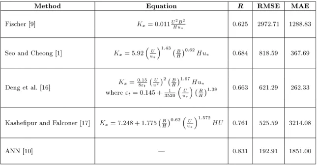
Initially four empirical models proposed by Fischer et al. [9], Seo and Cheong [1], Deng et al. [16], and Kashepour and Falconer [17] were applied to the complete dataset. The statistical performance evaluation measures like correlation coecient (R), Root Mean Square Error (RMSE), and Mean Absolute Error (MAE) are computed. The values of performance
evaluation measures for validation dataset for the four empirical models and ANN reported in the past are presented in Table 2. These results indicate that ANN method is found to be a successful tool for the prediction of longitudinal dispersion coecient in natural channels.
In this study an "-variant of SVM ("-SVM) is used for support vector regression and the loss function is xed as 0.001. The data mining software WEKA proposed by Witten and Frank [34] is used for devel-oping SVM model. Initially, a polynomial kernel of degree 2 is used to t a non-linear model. A trial and error approach is followed to nd the optimal value of kernel specic parameter C. The C parameter of 100 is found to be quite successful in giving satisfactory per-formance for validation dataset. The values of dierent performance evaluation measures for this model (for both training and validation dataset) are presented in Table 3. Table 3 shows that the RMSE value obtained for SVM with polynomial kernel for the validation dataset was better than those obtained by empirical approaches presented in Table 2. But the calculated R and RMSE values are not as good as those calculated for the results of ANN model. Then a Radial Basis Function (RBF) kernel is used to t a non-linear SVM
Table 2. Relative performance of empirical approaches and ANN.
Method Equation R RMSE MAE Fischer [9] Kx= 0:011UHu2B2 0.625 2972.71 1288.83
Seo and Cheong [1] Kx= 5:92
U u
1:43 B H
0:62Hu
0.684 818.59 367.69
Deng et al. [16] Kx=
0:15 8"t
U u
2 B
H
1:67Hu
where "t= 0:145 +35201
U u
B H
1:38 0.663 621.29 262.33
Kashepur and Falconer [17] Kx= 7:248 + 1:775 BH0:62
U u
1:572
HU 0.761 525.59 3214.08
Table 3. Performance evaluation of SVM and GP models.
Performance Training Testing Evaluation
Criteria
SVM Polynomial Kernel
(C = 100, d = 2)
SVM RBF Kernel (C = 100, = 3:5)
GP
SVM Polynomial Kernel
(C = 100, d = 2)
SVM RBF Kernel (C = 100, = 3:5)
GP
R 0.965 0.997 0.963 0.678 0.874 0.945 RMSE 38.59 11.30 41.64 461.40 106.09 60.44 MAE 20.93 4.33 24.71 174.99 79.27 54.42
model for the dataset. The combination of control parameters such as C = 100 and = 3:5 gives very good training performance. The dierent performance evaluation measures for RBF Kernel-based SVM is also (For both training and validation stages) summarized in Table 3.
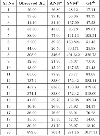
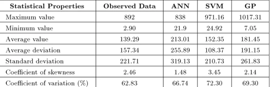
DISCIPULUS software proposed by Francone [35] is used for performing the GP-based modeling. The initial control parameters used for the problem are population size (500), crossover probability (0.95) and mutation probability (0.5). The basic arithmetical functions (such as addition, multiplication, subtraction and division (+, , , =) constitute the function set. The tness function is selected as the root mean square error between the measure and predicted values of longitudinal dispersion coecient. Based on the predicted values, three performance criteria namely R, RMSE and MAE are calculated and presented in Table 3. Table 3 shows that the GP-based model is better than both the ANN and SVM models. From Table 3, it can be seen that the performance evaluation measures of SVM (RBF Kernel) is better than those of GP. But the RBF Kernel shows inferior performance for the validation dataset. Thus it can be inferred that GP is able to capture the trend in a better way and it can be more generalized than SVM. The observed values, values predicted by ANN, RBF-based SVM and GP models for the testing dataset are presented in Table 4. The statistical properties such as maximum value, minimum value, average value, average deviation, stan-dard deviation, coecient of skewness, coecient of variation etc. are computed for observed data for validation and the values predicted, using dierent models, are presented in Table 5.
Table 5 shows that skewness and coecient of variation is the highest for SVM model; also both the extreme values are deviated largely from the observed extremes. This indicates that SVM is only fairly accurate in predictions. But the GP model results are better when compared with that of SVM.
The scatter plot of Kx between observed data
and the prediction of the best SVM model for only testing data group is presented in Figure 4. The 5% error bar lines are plotted along with in this scatter plot. Such a plot can be used to indicate the range
Table 4. The predicted and observed values of longitudinal dispersion by dierent models.
Sl No Observed Kx ANNa SVMb GPb
1 20.90 26.80 28.12 17.14 2 37.80 27.10 63.86 33.39 3 41.40 31.40 167.09 47.53 4 53.30 43.00 93.18 89.81 5 88.90 77.60 141.13 105.54 6 2.900 39.20 130.824 51.45 7 44.00 26.50 30.171 25.98 8 308.9 346.6 401.642 320.75 9 12.80 21.90 35.37 7.050 10 13.90 45.20 137.65 51.43 11 65.00 77.20 28.77 83.68 12 237.2 838.0 152.42 583.14 13 457.7 838.0 153.09 379.58 14 374.1 838.0 152.42 518.00 15 41.80 59.70 132.08 169.74 16 10.70 26.90 24.92 24.17 17 36.90 76.60 66.91 70.28 18 15.50 25.30 42.32 14.60 19 30.20 31.70 93.97 18.49 20 892.0 763.4 971.16 1017.31
a: Tayfur and Singh [10]. b: Present study.
of standard deviation and to determine whether the dierences are statistically signicant [36]. A similar plot for the best GP model for the testing dataset is presented in Figure 5. From the plots also it can be inferred that for the GP model more data points in the prediction dataset falls within the 95% condence interval when compared with those obtained by SVM. DISCUSSION
The dierent performance evaluation criteria calcu-lated for the testing data based on ANN model results by Tayfur and Singh [10] established that ANN-based modeling is superior to the existing theoretical and
em-Table 5. Statistical properties of values predicted by dierent models. Statistical Properties Observed Data ANN SVM GP Maximum value 892 838 971.16 1017.31 Minimum value 2.90 21.9 24.92 7.05 Average value 139.29 213.01 152.35 181.45 Average deviation 157.34 255.89 108.37 191.15 Standard deviation 221.71 319.13 210.73 261.83 Coecient of skewness 2.46 1.48 3.45 2.14 Coecient of variation (%) 62.83 66.74 72.30 69.30
Figure 4. The 5% error bar for SVM model (RBF Kernel).
Figure 5. The 5% error bar for GP model.
pirical equations. However, ANN modeling involves the tedious process of optimal setting of a larger number of control parameters such as number of hidden layers, learning rate, momentum rate, number of iterations, transfer function and weight initialization. The results
show that SVM modeling with RBF kernel show better prediction of longitudinal dispersion coecient than those with ANN modeling.
The results of GP-based modeling for testing dataset show that it captures the non linearity of the dataset quite well. It gives a correlation coecient value of 0.945 for testing dataset and the RMSE value of 60.44 and MAE of 54.42 which is the lowest when compared with the results by empirical equations, ANN and SVM. The dierent performance evaluation measures show that SVM predicts the values of Kx
very well for the training dataset but the prediction accuracy is not as good as that of GP (Table 3).
This establishes the better generalization capa-bility of GP when compared with SVM. Moreover the GP-based modeling follows a progressive improvement towards the global optima (i.e., minimum error) and give the output in the form of a computer program which is quite useful for the modeler to apply for a new set of input data for predicting the longitudinal disper-sion coecient. Thus the present study establishes the potential of GP in accurate prediction of longitudinal dispersion coecient in natural channels. The sensitiv-ity analysis with a modied procedure establishes that the bed width of the channel as the most signicant parameter which aects the longitudinal dispersion and the results are on the expected lines.
CONCLUSION
In this paper the application of two relatively recent soft computing techniques - SVM and GP are investi-gated for the prediction of longitudinal dispersion coef-cient in natural channels. SVM predicts longitudinal dispersion coecient quite well when compared with the empirical approaches and ANN. Also it demands the optimal selection of only a few number of control parameters when compared with ANN. Performance evaluation based on multiple error criteria show that the two error criteria (RMSE and MAE) are the least and correlation coecient (R) is the highest for the GP-based modeling than any other model considered in this study. The GP-based modeling is found to be superior
in terms of quality and it gives the output in the form of computer programs which enables the user to apply for a new set of input data to predict the longitudinal dispersion coecient. Thus GP can be recommended as a robust soft computing paradigm to predict the longitudinal dispersion coecient in natural channels. REFERENCES
1. Seo, I.W. and Cheong, T.S. \Predicting longitudinal dispersion coecient in natural streams", Journal of Hydraulic Engineering, ASCE, 124(1), pp. 25-32 (1998).
2. Li, Z.H., Huang, J. and Li, J. \Preliminary study on longitudinal dispersion coecient for three gorges reservoir", in Proceedings of the Seventh International Symposium Environmental Hydraulics, Hong Kong, China (Dec. 16-18, 1998).
3. Fischer, B.H., List, E.J., Koh, R.C., Imberger, J. and Brookes, N.H., Mixing in Inland and Coastal Waters, Academic, New York (1979).
4. Seo, I.W. and Baek, K.O. \Estimation of longitudinal dispersion coecient using velocity proles in natural streams", Journal of Hydraulic Engineering, ASCE, 130(3), pp. 227-236 (2004).
5. Sedighnezhad, H., Salehi, H. and Mohein, D. \Com-parison of dierent transport and dispersion of sed-iments in Mard intake by FASTER model", in Pro-ceedings of the Seventh International Symposium River Engineering, Ahwaz, Iran, pp. 45-54 (Oct. 16-18, 2007).
6. Taylor, G.I. \Dispersion of soluble matter in solvent owing slowly through a tube", Proc. Royal Society of London, Sec A, 219, pp. 186-203 (1953).
7. Taylor, G.I. \Dispersion of matter in turbulent ow through a pipe", Proc. Royal Society of London, Sec A, 223, pp. 446-468 (1954).
8. Elder, J.W. \The dispersion of a marked uid in turbulent shear ow", Journal of Fluid Mechanics, Cambridge University Press, 5(4), pp. 544-560 (1959). 9. Fischer, B.H. \The mechanics of dispersion in natural streams", Journal of Hydraulic Division, ASCE, 93(6), pp. 187-216 (1967).
10. Tayfur, G. and Singh, V.P. \Predicting longitudinal dispersion coecient in natural streams by articial neural network", Journal of Hydraulic Engineering, ASCE, 131(11), pp. 991-1000 (2005).
11. Toprak, Z.F. and Cigizoglu, H.K. \Predicting longi-tudinal dispersion coecient in natural streams by articial intelligence methods", Hydrological Processes, Wiley, 22, pp. 4106-4129 (2008).
12. Toprak, Z.F. and Savci M.E. \Longitudinal dispersion modeling in natural channels by fuzzy logic", CLEAN-Soil, Air, Water, Wiely, 35(6), pp. 626-637 (2007). 13. Madvar, H.R., Ayyoubzadeh, S.A., Khadangi, E. and
Ebadzadeh, M.M. \An expert system for predicting
longitudinal dispersion coecient in natural streams by using ANFIS", Expert Systems with Applications, Elsevier, 36, pp. 8589-8596 (2009).
14. Tayfur, G. \GA optimized model predicts longitudinal dispersion coecient in natural channels", Hydrology Research, 40(1), pp. 60-78 (2009).
15. Samui, P. \Prediction of friction capacity of driven piles in clay using the support vector machine", Cana-dian Geotechnical Journal, 45, pp. 288-295 (2008). 16. Deng, Z.Q., Singh, V.P. and Bengstsson, L.
\Longitu-dinal dispersion coecient in straight rivers", Journal of Hydraulic Engineering, ASCE, 127(11), pp. 919-927 (2001).
17. Kashepour, M.S. and Falconer, R.A. \Longitudinal dispersion coecient in natural channels", Water Re-search, Elsevier, 36(6), pp. 1596-1608 (2002).
18. Boser, B.E., Guyon, I.M. and Vapnik, V.N. \A training algorithm for optimal margin classiers", 5th Annual ACM Workshop on Colt, D. Haussler, Ed., Pittsburgh, PA: ACM Press, pp. 144-152 (1992).
19. Vapnik, V.N., The Nature of Statistical Learning The-ory, Springer, New York (1995).
20. Cortes, C. and Vapnik, V.N. \Support vector net-works", Machine Learning, Springer, 20, pp. 273-297 (1995).
21. Smola, A.J. and Scholkopf, B. \A tutorial on support vector regression", Statistics and Computing, Springer, 14, Doi: 10.1023/B:STCO.0000035301.49549.88, pp. 199-222 (2004).
22. Vapnik, V.N., Statistical Learning Theory, Wiley, New York (1998).
23. Pal, M. and Goel, A. \Prediction of the end-depth ratio and discharge in semi-circular and circular shaped channels using support vector machines", Flow Mea-surement and Instrumentation, Elsevier, 17, pp. 49-57 (2006).
24. Rajasekharan, S., Gayathri, S. and Lee, T.L. \Support vector regression methodology for storm surge predic-tions", Ocean Engineering, Elsevier, 35, pp. 1578-1587 (2008).
25. Goel, A. and Pal, M. \Application of support vector machines in scour prediction on grade control struc-tures", Engineering Applications of Articial Intelli-gence, Elsevier, 22(2), pp. 216-223 (2009).
26. Holland, J.H., Adaptation in Natural and Articial Systems, Ann Arbour Science Press, Ann Arbour, USA (1975).
27. Goldberg, D.E., Genetic Algorithms in Search, Op-timization and Machine Learning, Addison-Wesley (1989).
28. Koza, J.R., Genetic Programming: On the Program-ming of Computers by Means of Natural Selection, MIT Press, Cambridge, MA, USA (1992).
29. Khu, S.T., Liong, S.Y., Babovic, V., Madsen, H. and Muttil, N. \Genetic programming and its application
in real time runo forecasting", Journal of American Water Resource Association, Wiley, 37(2), pp. 439-451 (2001).
30. Savic, D.A., Walters, A. and Davidson, J.W. \A genetic programming approach to rainfall runo mod-eling", Water Resource Management, Springer, 13, pp. 219-231 (1999)
31. Babovic, V. \Data mining and knowledge discovery in sediment transport", Computer Aided Civil and Infrastructural Engineering, Wiley, 15(5), pp. 383-389 (2000)
32. Whigham, P.A. and Crapper, P.F. \Modelling rainfall-runo using genetic programming", Mathematical and Computer Modeling, Elsevier, 33, pp. 707-721 (2001). 33. Azmathullah, H.Md., Ghani, A.A.B., Zakaria, N.A., Lai., S.H., Chang, C.K., Leow, C.S. and Abuhasan, Z. \Genetic programming to predict sky-jump bucket spillway scour", Journal of Hydrodynamics, Elsevier, 13(4), pp. 477-484 (2008).
34. Witten I.H. and Frank, E., Data Mining, Morgan Kaufmann, San Francisco (2000)
35. Francone, F.D., Discipulus Owner's Manual, version 3.0 DRAFT, Machine Learning Technologies Inc. Lit-tleton, CO, USA (1998).
36. Samui, P. and Sitharam, T.G. \Lest square support vector machines applied to settlement of shallow foun-dations on cohesionless soils", International Journal for Numerical and Analytical Methods in Geomechan-ics, Wiley, Doi: 10.1002/nag.731 (2008).
BIOGRAPHY
Sankaran Adarsh completed the graduation in Civil Engineering from TKM College of engineering Kol-lam, Kerala, India in 2003, and masters degree in Water Resources Engineering from Indian Institute of Technology Bombay (IITB), India, in 2009. He is presently working as a lecturer in the Department of Civil Engineering TKM College of Engineering Kollam, Kerala, India and having more than 6 years experi-ence in teaching and consultancy. He has published research articles in four international journals and two conferences. His area of interests are Optimization of Hydrosystems using Stochastic Search Algorithms, Predictive Modeling in Water Resources and Hydrology using Soft Computing Techniques and Hydroclimatol-ogy.